Reinforcement Learning Primer

Reinforcement learning is going to be “the next big thing” in machine learning after 2022, so let’s understand some basic on how it works.

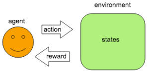
• Agent: trying to make decision
• Environment: everything outside the agent

Supervised, unsupervised, and reinforcement learning

People like to classify machine learning into these 3 categories

• Supervised learning: the model can train with label of what is expected to predict the label from features
• Unsupervised learning: the model has no label to train and is expected to learn some structure about the data via the features
• Reinforcement learning: the model does not have direct label to train but can interact with the “environment” by taking actions and observations, and the model is expected to learn how to optimally behave in the environment to maximize some reward

Terminology

• A_t: action at time t
• R_t: reward at time t

Reward function

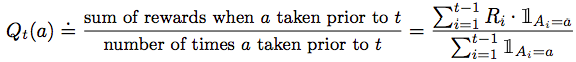
The expected reward function at time t with action a is a function of the action at time t

Note that this function is not given to the agent in the reinforcement learning framework. It’s learned about the model.

• This is bad because it makes it hard for the agent to make decision on the action not knowing the expected reward function
• This is good because it’s often hard to find this function anyway and we can let the agent learn this function from the data

The estimated reward function at time t is denoted by Q(a) a time t

This function is what the agent has to work with because it does not know q*. The goal is to have Q() be close to q*() as much as possible.

Exploration and Exploitation

• Exploitation:
  • Taking the best action a that maximize the one-step reward using Q()
  • This is optimal move if there is only one move left to make (greedy)
• Exploration:
  • Taking anything that is not the best action
  • Help to refine Q() so that the agent understands the true expected reward function better
  • Better Q() means high chance of making the best decision in the future
  • This is optimal when there are many moves left to make and the agent has high uncertainty on the expected reward (there might another action that could have higher reward)

Traditionally there are some way to solve for the “best” strategy to balance exploration and exploitation by making assumption about the prior knowledge and stationarity of the problem. But this is not practical in most situation, so RL is basically a way to more adaptively balance exploitation and exploration to achieve maximum total reward at the end.

Action-value Methods

Action-value Methods refer a collection of methods to (1) estimate the value of actions and (2) make decision based on the estimates.

The expression for Q above simply means just take the sample average of historical reward for each action a as an estimate of what the expected reward should be for taking action a. As t goes to infinity, we expect Q converges to q*.

For a given action a, which has been selected n times, we have the sample average reward as

To compute this efficiently at each time this action is selected, we can use an incremental update rule

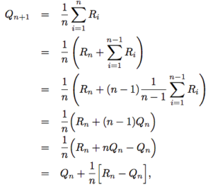
This form is very commonly used where we call the 1/n a “step size” and make it a configurable parameter later.

The greedy action is the optimal a that maximizes Q at a given t.

Of course, we cannot just behave greedily at the time. One simple strategy is to act greedily most of the time but explore other actions with small probability epsilon. In the long run, as we Q approximates q* very well, the agent will be behaving optimally 1-epsilon probability of the time.

Multi-Armed Bandit Problem

To get started with the simplest set up of an reinforcement learning problem, see Multi-Armed Bandit Problem

Non-stationary problem

When the mean of each bandit can change over time, the agent needs to be adapt with incremental update rule

where alpha is between 0 and 1. It can also be rewritten as below

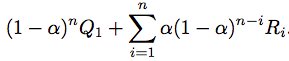
This shows that Qn depends on Q1 (aka Initial Action Value) and all to previous Rewards. These weights sum up to 1. So this is also called the exponential recency-weighted average.

Reference: most of the material of this post comes from the book Reinforcement Learning

To learn more about RL:

• Reinforcement Learning Glossary
• Multi-Armed Bandit Problem
• Finite Markov Decision Processes (MDP)
• Solving MDPs with dynamic programming
• Planning with Tabular Methods in Reinforcement Learning
• Monte Carlo Methods in RL
• Temporal Difference Learning
• Temporal Difference Control in Reinforcement Learning
• Approximate Function Methods in Reinforcement learning
• Reinforcement learning: policy gradient methods