Policy gradient methods are a type of Reinforcement Learning optimization methods that works by performing gradient ascent on the parameters of a parameterized policy. This is in contrast with the action-value methods which usually maintains a table of action or action-state values and then choose action by choose (greedily or epsilon-greedy) action based on those values.
Parameterized Policy
- In action-value methods, a policy is typically denoted as pi(state, action) whether it’s deterministic or stochastic
- In policy gradient methods, a parameterized policy is denoted as pi(action | state, theta). Theta is the parameter vector of the policy. It is possible to generalize a parameterized policy as an action-value function by using the parameter vector to represent the action-value table.
Why do we need a parameterized policy?
- In some cases, policy parameterization may be a simpler function to approximate than the action-value methods
- It will help the problem to learn fast if we can use a simpler policy and more optimal policy.
- In other cases, if the action-value function is simpler, then the problem can learn faster and better with action-value function.
- Most important reason: policy parameterization is that it’s a good way to inject prior knowledge about the desired form of the policy into the reinforcement learning system.
Learning value function
Policy gradient might or might not use a value function. Typically it would be an estimated value function denoted as v_hat(state, weight)
Policy Gradient
The performance under parameter vector theta is denoted by J(theta), then the performance gradient is basically taking the gradient of J w.r.t theta.
We then perform gradient ascent on theta.
![]()
Note that “hat” on the gradient is due to the stochastic nature that we can almost never get the true gradient but use our observation to estimate the gradient.
Requirement on the policy pi(a | s, theta)
- The gradient of the policy pi(action | state, theta) needs to be differentiable w.r.t theta.
- The policy should not be determinist to ensure exploration which means pi(a | s, theta) should be strictly with in (0, 1) for all a, s, theta.
For action space that is discrete and not too large, a natural parameterization is to apply soft-max over the action preference function h(s, a, theta)
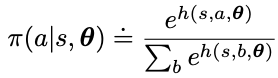
The action preference function h(s, a, theta) can be arbitrary (ie, neural network) or simply a linear function of theta over the feature vectors
This function has the nice properties
- Soft-max represents probability and ensuring exploration.
- The stochastic policy can approximate a deterministic policy. In fact, if the optimal policy is deterministic, the action preference of certain state-action pairs will be driven to infinity to prefer over all sub-optimal actions
- We can add temperature to let the stochastic policy to converge to a deterministic policy over time
- In problem with significance function approximation, the best policy might be stochastic. (Ex. poker game that requires bluffing) Action-value methods have no natural way of finding stochastic optimal policies, whereas policy approximating methods can.
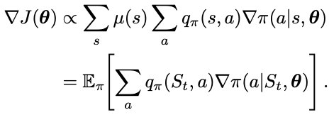
Policy Gradient Theorem
There is a theoretical advantage of the policy parameterization over epsilon-greedy action selection is smoothness. With continuous parameterization (theta being continuous), the action probability is changing smoothly as well, but for epsilon-greedy action selection could be changing the action probabilities abruptly to result in a large changing in the value. This gives stronger convergence guarantee for policy gradient methods than action-value methods. This guarantee makes approximate gradient ascent possible in policy gradient methods.
Challenge of policy gradient: given a state, the effect of the policy parameter on the actions and reward is easy to compute, but the effect of the policy on the state distribution is a function of the environment and is typically unknown. How can we estimate the performance gradient with respect to the policy parameter when the gradient depends on the unknown effect of policy changes on the state distribution? This is precisely what the policy gradient theorem answers:
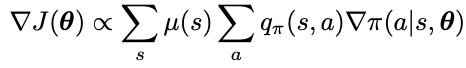
- mu is the on-policy state distribution under the policy pi
- pi is the policy under parameter vector theta
- it does not involve the derivative of the state distribution
- the proportional sign is used here because for episodic case the constant is the average length of an episode, and for continuing case the constant is 1
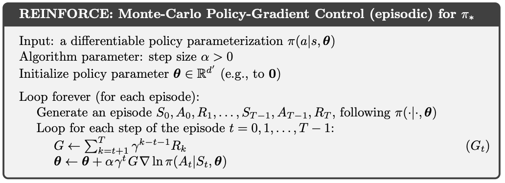
Monte Carlo Policy Gradient (episodic and no discounting)
One way to estimate the true performance gradient over the policy parameters is to use samples. The samples need to have expected value that is proportional to the true gradient since the constant is absorbed into the step size. Rewriting the performance gradient as an expectation, we have
Using the expression inside the expectation, we have the Monte Carlo Policy Gradient update formula as
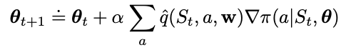
where q_hat is the learned approximation of the true value function under policy pi. This is called an all-actions methods because the update affects all actions. To sample this value requires summing up over all actions. This might be time consuming in some cases. So one more is to break down the performance gradient further to have an update function that only affects just one action each time.
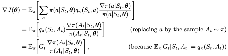
- By introducing a weighting factor “grad pi(A_t | S_t, theta) / pi(A_t | S_t, theta), we allow the sum of all actions a to be absorbed away in the expectation expression under policy pi
- We changed the expectation from sampling over the state S_t to the sampling over action A_t
- G_t is the return at time step t
This yields the final update formula for the classical REINFORCE algorithm:
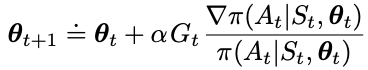
- The increment consists of 3 components: the return, the gradient of the probability of action A_t over theta, and the probability of action A_t
- The direction of the gradient in parameter space points to the most increase of the probability of repeating the action A_t on future visits to state S, and this is scaled by the return
- The denominator is inversely scaled by the probability of the action to offset the fact that the action is already selected frequently at an advantage.
- This makes good intuitive sense because we only want to update to promote an action by as much as its future return but also inversely by its current probability
- To estimate G_t, we still need the complete future return from time step t, so this is still a Monte Carlo method and works well for episodic cases.
- Note that grad ln( pi( A_t | S_t, theta) is used here because of the logarithmic derivate: “grad ln x = grad x / x”
- The above gradient vector is also known as the eligibility vector
- Note that discount factor gamma is reintroduced by to the algorithm for completeness
- Because of the stochastic gradient is estimated by MC, there is still a high variance problem and learning/convergence can be slow.
REINFORCE with a baseline
One trick to improve the REINFORCE method above is to use a base line to reduce the variance.
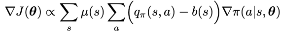
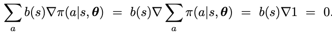
The baseline b(s) can be any function or random variable (cannot depend on action a). We can show the below that the baseline should not impact the policy gradient because when summed over the entire action space of a policy, then gradient of total probability of 1 is 0.
The baseline depends on the state S_t, and we have another update formula
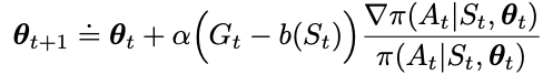
One choice of the baseline function b(S_t) can be a the estimated value function using weight vector w on the features, in which we denote as v_hat(S_t, w)
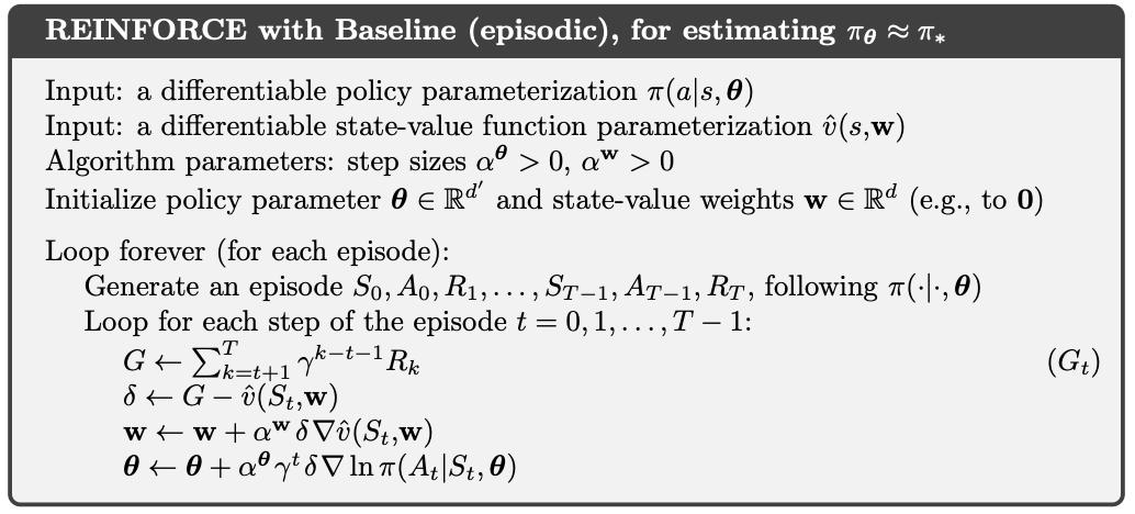
- Note the two separate step sizes for w and theta
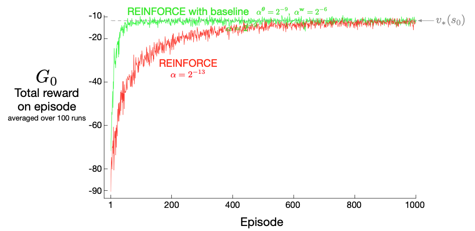
- See much faster convergence in the short-corridor gridworld example
Actor-Critic
When we learn the parameters of a policy directly, does it mean we cannot learn the value function? No, even in policy gradient methods, value-learning methods like TD is still important. Policy gradient methods that use learn approximations to both policy and value functions are often called actor–critic methods
- actor: the learned policy
- critic: the learned value function, usually a state-value function (not state-action-value function) to evaluate the actions by the actor
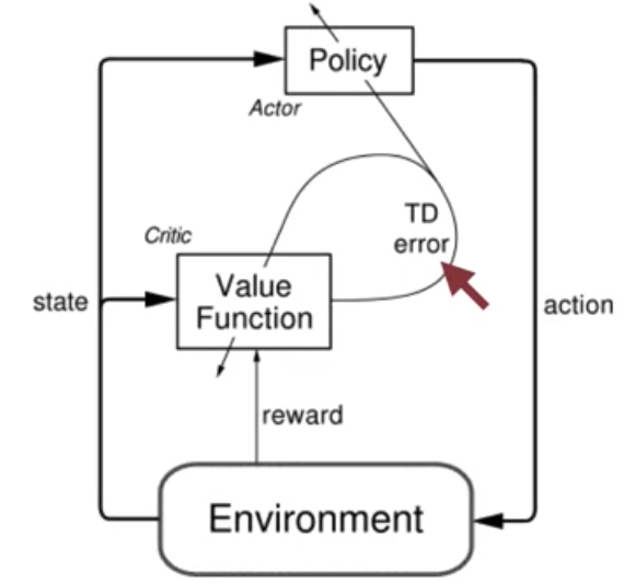
We use the TD error to update both the policy and value function in each iteration.
Bootstrapping
Even though the REINFORCE with a baseline uses the state-value as a baseline, we don’t consider it an actor-critic method. To be a critic, we mean bootstrapping (updating the value estimate for a state from the estimated values of subsequent states). The distinction here is that in bootstrapping we introduce bias and an asymptotic dependence on the quality of the function approximation. In contrast, the Monte Carlo method above does not have any bias, and whatever baseline we use does not cause a difference in asymptotic behavior.
Why do we even what the bias then? It turns out be beneficial in reducing variance and accelerating learning (Think temporal-difference vs MC).
One step actor-critic
The main appeal of one-step methods is that they are fully online and incremental, yet avoid the complexities of eligibility traces. One-step actor-critic methods replace the full return (G_t)
of REINFORCE with the one-step return (and use a learned state-value function as the baseline)
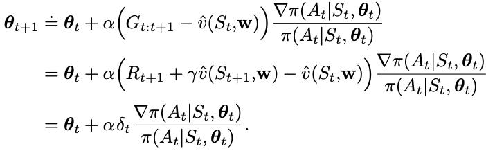
To understand the last step intuitively, it changes the policy parameters to increase the probability of actions that were better than expected according to the critic.
- The probability gradient is captured as “grad pi( action | state, theta )”
- The amount of improvement in the return is captured by delta_t
- Alpha is the step size specific for updating theta.
This makes it fully online, incremental algorithm, with states, actions, and rewards processed as they occur and then never revisited.
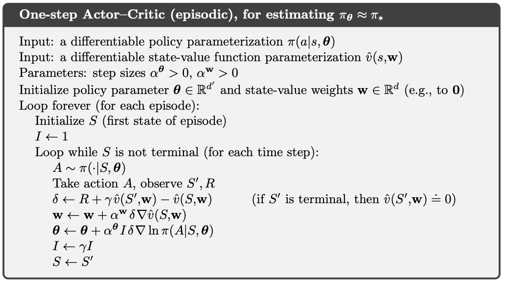
The key variable is delta (TD error)
- R is immediately observed reward, hence we have “one-step” method
- gamma is the discount factor
- v_hat( current state, weight ) is the estimated return from the observed current state
- w is the weight vector of the state-value function
- v_hat( previous state, weight ) is the estimated return from the previous state to be used as a baseline
- The expected value of the policy parameter gradient does not change since the expectation under the policy pi on v_hat( prev state, w ) * (grad ln pi ( action | prev state, theta ) ) = 0
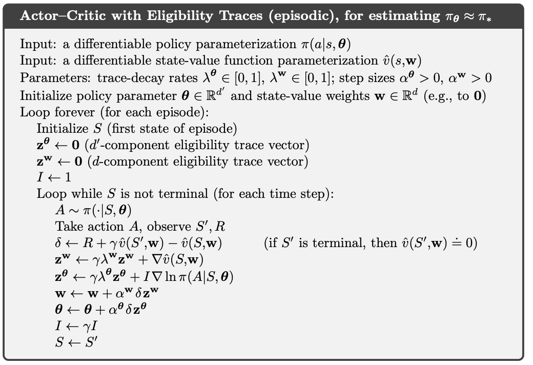
It can be generalized to the forward view of n-step methods and then to a lambda-return algorithm, but need to learn about eligibility trace.
Actor-critic for Continuing cases
- In episodic cases, the performance is defined as the value of the start state under the parameterized policy
- In continuing cases, the performance is defined as the average reward rate
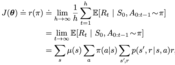
Using backward view for the continuing case,
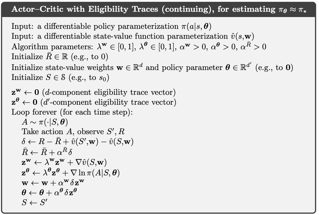
The key variable is delta (TD error)
- R_bar is used because we are using average reward, which is calculated by taking an special form of exponential averaging of the delta
- v_hat( current state, weight ) is the estimated return from the observed current state
- w is the weight vector of the state-value function
- v_hat( previous state, weight ) is the estimated return from the previous state to be used as a baseline
Reference: most of the material of this post comes from the book Reinforcement Learning