NLP Tutorial: Named Entity Recognition using LSTM and CRF

Introduction

Named Entity Recognition (NER) is a very classic natural language processing (NLP) problem. The task is to identify the words in a sentence that represents named entities.

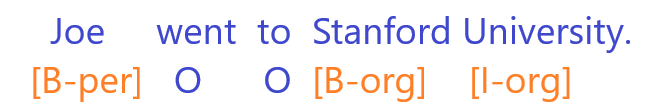
For example, if we are given a sentence: Joe went to Stanford University.

We expect to recognize the two named entities: (1) Joe and (2) Stanford University.

More specifically we want to identify the types of entity as well (ie whether it’s a person or location). We are going to use the Inside–outside–beginning (IOB) format for tagging entities.

First part differentiates the beginning (B), inside (I), and outside of entities.

Second part represents the type of entity

geo = Geographical Entity
org = Organization
per = Person
gpe = Geopolitical Entity
tim = Time indicator
art = Artifact
eve = Event
nat = Natural Phenomenon

How (some math background)

Historically, this is done using a predefined as of words that are known to be named entity. For example, the word Joe is the name of a person, and the Stanford University is the name of a school. However, this is difficult because a word can appear in different forms. For example,

• Roger is a tennis player.
• Roger that!

In these two sentences, the word Roger is a person in the first sentence but an exclamation in the second sentence. This will be hard to handle as you would require even more complex rules to class it. Wouldn’t it be better if you have apply statistics to train a model that can learn these patterns?

One of a statistical method is to use a linear chain conditional random field (CRF) model to learn the probablistic model to find the mostly probable tagging for the sentence. In combination we use a bidirectional long shorter term memory (LSTM) model to process the input sequence into a compressed hidden states.

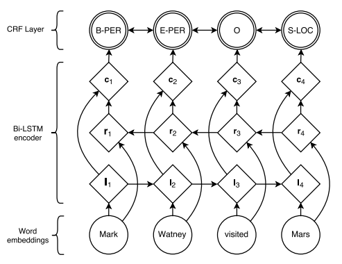
Let’s look at the diagram layer from Neural Architectures for Named Entity Recognition

• At the bottom layer, we have word embedding. We can either train our own embedding or use a pretrained embedding layer. In this tutorial, we will train our low dimensional embedding, but in practice, it might be worth using an existing pretrained word embedding.
• Next layer up is the Bi-LSTM, which can be viewed as a encoder to transfrom the embedding to another representation that takes the context in account because LSTM is a sequence model that passes the hidden states from previous and and next word using the bidrectional layers by concatenating the output of both directions as one vector for each word. At this layer, it’s already possible to build a POS tagging model by mapping the output two output a softmax layer to output to predict the tags, such model will effectively be independent predicting the tag for each word without using any grammar. By grammar, I mean modelling the conditional probability among the words. Thus, we try to do more with a CRF layer in this tutorial.
• At the out of the LSTM encoder, we have the encoded representation which are passed to the CRF layer as input. You can also skip to the end to see how CRF layer work mathamatically.

Coding

Now let’s get into how to do it in a colab.

First I ran the below pip install commands in my colab. This really depends on your colab environment. At the time of this article (2022), I had to specific the tensorflow and keras version to make sure the CRF layer can work properly.

!pip install tensorflow==2.2 
!pip install keras==2.3.1
!pip install plot-keras-history
!pip install git+https://www.github.com/keras-team/keras-contrib.git
!pip install tensorflow_addons

Import as usual…

import pandas as pd
import numpy as np
import matplotlib.pyplot as plt

from plot_keras_history import plot_history
from sklearn.model_selection import train_test_split
from sklearn.metrics import multilabel_confusion_matrix, confusion_matrix

import tensorflow as tf 
import keras

from keras import layers
from keras import optimizers

from keras.models import Model
from keras.models import Input

from keras_contrib.layers import CRF
from keras_contrib import losses
from keras_contrib import metrics

import seaborn as sn
from matplotlib.colors import LogNorm

Download data

Read the training data from csv. You can download the csv from kaggle.

Download link: https://www.kaggle.com/datasets/abhinavwalia95/entity-annotated-corpus

I have download my data so I can just load it from my Google Drive:

from google.colab import drive
drive.mount('/content/drive')
file_path = "/content/drive/MyDrive/kaggle_ner_dataset/ner_dataset.csv"
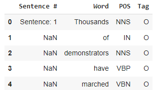
df = pd.read_csv(file_path, encoding="iso-8859-1", header=0)
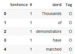
df.head()

Data Processing

• We see the first column “Sentence #” is used to denote which sentence the word is in, but it’s a string, so we need to convert the sentence number from string to int
• Since only the first word of every sentence has the sentence number label while the rest has NaN. We use ffill (forward fill) to copy it to all records after the labeled record for each sentence.

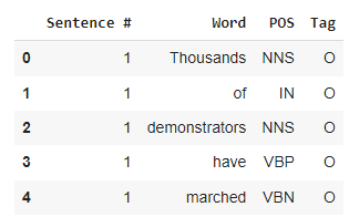
df = df.fillna(method="ffill")

# Extra the substring after "Sentence: "
df["Sentence #"] = df["Sentence #"].apply(lambda s: int(s[9:]))
df.head()

For this time, we don’t need the POS tag, so let’s just remove this column.

Note: this POS data can be also useful for training a Hidden Markov Model for POS Tagging

df.drop('POS', axis=1, inplace=True)
df.head()

Exploratory Data Analysis

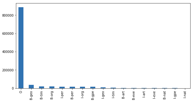
df["Tag"].value_counts().plot(kind="bar", figsize=(10,5));

df[df["Tag"]!="O"]["Tag"].value_counts().plot(kind="bar", figsize=(10,5))

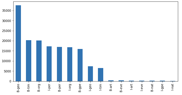
We can see here that geography names, time, organization names are very popular.

The tag notation has two parts

First part differentiates the beginning (B) and the inside (I) of entities.

Second part represents the type of entity

• geo = Geographical Entity
• org = Organization
• per = Person
• gpe = Geopolitical Entity
• tim = Time indicator
• art = Artifact
• eve = Event
• nat = Natural Phenomenon

We also want to check the length of the sentences in the dataset because we need to decide how to set up the max length in our model later.

word_counts = df.groupby("Sentence #")["Word"].agg(["count"])
word_counts.hist(bins=50, figsize=(8,6));

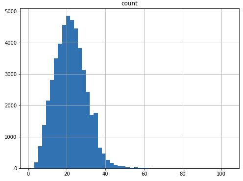
As we can see, the average lenght is around 20 but it has a long tail on the right.

max_length=word_counts.max()

To speed up the training, let’s only process the shorter sentences for demo purpose. You are free to skip this part of the code if you want to process all sentences.

max_length=70
print("There are {} sentences over {} words.".format(np.sum(word_counts['count']>max_length), max_length))

There are 4 sentences over 70 words.

keep_sentence_ids = word_counts[word_counts['count']<=max_length].index
df = df[df['Sentence #'].isin(keep_sentence_ids)]

Converting words and TAGs to numerical values

We need to build dictionary to convert between string and numbers because the keras model that we use needs to accept numeric tensors.

all_words = list(df["Word"].unique())
all_tags = list(df["Tag"].unique())

Let’s build two dictionary to convert between the words in string to index.

word2index = {word: idx for idx, word in enumerate(all_words, 2)}

# Setup the reserved index 0 and index 1 for two special tokens: unknown word and padding
word2index["<_UNK_>"]=0
word2index["<_PAD_>"]=1

# Create the inverted dictionary
index2word = {idx: word for word, idx in word2index.items()}

• We can take a quick look at the dictionary
• Get word from index
• Get index from word
• Confirm the index is same as after mapping thru both index2word and word2index

for i in range(5):
  word = index2word[i]
  index = word2index[word]
  print("i={} word={:10s} index={}".format(i, word, index))

i=0 word=<_UNK_>       index=0 
i=1 word=<_PAD_>       index=1 
i=2 word=Thousands     index=2 
i=3 word=of            index=3 
i=4 word=demonstrators index=4

Next, build 2 dicinotaries to convert between the TAG and index.

tag2index = {tag: idx for idx, tag in enumerate(all_tags, 1)}

# Setup the reversed index 0 for padding in the TAG sequence
tag2index["<_PAD_TAG_>"] = 0

# Create the inverted dictionary
index2tag = {idx: word for word, idx in tag2index.items()}

Each word in the data set has a corresponding tag, but they are in separate columns in the data set. So we apply two operations to bring the data to the right form:

• Group the data by sentence #
• Convert the 2 columns to 2 lists and zip the 2 lists into 1 list of triples for each sentence.

listOfListOfWords = df.groupby("Sentence #")['Word'].apply(lambda x: x.values.tolist()).tolist()
listOfListOfTags = df.groupby("Sentence #")['Tag'].apply(lambda x: x.values.tolist()).tolist()

print(listOfListOfWords[0])
print(listOfListOfTags[0])

['Thousands', 'of', 'demonstrators', 'have', 'marched', ...]
['O', 'O', 'O', 'O', 'O', 'O', 'B-geo', 'O', 'O', 'O', ...]

X = [[word2index[word] for word in listOfWords] for listOfWords in listOfListOfWords]
y = [[tag2index[tag] for tag in listOfTags] for listOfTags in listOfListOfTags]

# Convert the sentences from string to index and pad to max length
X = [listOfWordIndices + [word2index["<_PAD_>"]] * (max_length - len(listOfWordIndices)) for listOfWordIndices in X]
# Convert the tags from string to index and pad to max length
y = [listOfTagIndices + [tag2index["<_PAD_TAG_>"]] * (max_length - len(listOfTagIndices)) for listOfTagIndices in y]
print(X[0])
print(y[0])

[2, 3, 4, 5, 6, 7, 8, 9, 10, 11, 12, 13, 14, 15, 16, 11, 17 ...]
[1, 1, 1, 1, 1, 1, 2, 1, 1, 1, 1, 1, 2, ...]

Next we need to turn the densely encoded label of tags to one-hot encoding.

num_tags = len(index2tag)
y = [np.eye(num_tags)[listOfTagIndices] for listOfTagIndices in y]

Convert the data to numpy arrays and split into train and test sets

X_train = np.array(X_train)
X_test = np.array(X_test)
y_train = np.array(y_train)
y_test = np.array(y_test)


print("X_train:", X_train.shape)
print("X_test:", X_test.shape)
print("y_train:", y_train.shape)
print("y_test:", y_test.shape)

X_train: (43159, 70) 
X_test: (4796, 70) 
y_train: (43159, 70, 18) 
y_test: (4796, 70, 18)

Model

The model we want to build is the LSTM-CRF from Neural Architectures for Named Entity Recognition

vocab_size = len(index2word)
print(vocab_size, vocab_size ** 0.25)

35164 13.693818515221722

As a rule of thumb by Google, we choose dense embedding dimension to be 14.

input_layer = layers.Input(shape=(max_length,))
model = layers.Embedding(vocab_size, 14, embeddings_initializer="uniform", input_length=max_length)(input_layer)

# Drop out of 0.1 is used for extra robustness (the paper used 0.5)
# LSTM hidden state has dimension of 50 as suggested in the paper.
# return_sequences = True because we want pass the output from all time steps to the next layer
model = layers.Bidirectional(layers.LSTM(50, recurrent_dropout=0.2, return_sequences=True))(model)

# Connect a Dense layer to the output of the Bidirectional LSTM to output at dimension of 100 as suggested in the paper.
model = layers.TimeDistributed(layers.Dense(100, activation="relu"))(model)

# The CRF layer is the output layer and it should have the matching output dimension as the number of tags.
crf_layer = CRF(units=num_tags)
output_layer = crf_layer(model)

ner_model = Model(input_layer, output_layer)

# Need to apply the specific loss objective and accuracy metric for the CRF layer
loss = losses.crf_loss
acc_metric = metrics.crf_accuracy
ner_model.compile(optimizer=tf.optimizers.Adam(lr=0.001), loss=loss, metrics=[acc_metric])

ner_model.summary()

Model: "model_1"
_________________________________________________________________
Layer (type)                 Output Shape              Param #   
=================================================================
input_1 (InputLayer)         (None, 70)                0         
_________________________________________________________________
embedding_1 (Embedding)      (None, 70, 14)            492296    
_________________________________________________________________
bidirectional_1 (Bidirection (None, 70, 100)           26000     
_________________________________________________________________
time_distributed_1 (TimeDist (None, 70, 100)           10100     
_________________________________________________________________
crf_1 (CRF)                  (None, 70, 18)            2178      
=================================================================
Total params: 530,574
Trainable params: 530,574
Non-trainable params: 0
_________________________________________________________________

history = ner_model.fit(X_train, y_train, batch_size=256, epochs=20, validation_split=0.1, verbose=2)

Train on 38843 samples, validate on 4316 samples
Epoch 1/20
 - 54s - loss: 0.5942 - crf_accuracy: 0.8606 - val_loss: 0.2495 - val_crf_accuracy: 0.9499
Epoch 2/20
 - 53s - loss: 0.2222 - crf_accuracy: 0.9509 - val_loss: 0.1734 - val_crf_accuracy: 0.9516
Epoch 3/20
 - 48s - loss: 0.1259 - crf_accuracy: 0.9615 - val_loss: 0.1054 - val_crf_accuracy: 0.9679
Epoch 4/20
 - 49s - loss: 0.0907 - crf_accuracy: 0.9732 - val_loss: 0.0842 - val_crf_accuracy: 0.9769
Epoch 5/20
 - 48s - loss: 0.0683 - crf_accuracy: 0.9815 - val_loss: 0.0649 - val_crf_accuracy: 0.9833
Epoch 6/20
 - 48s - loss: 0.0511 - crf_accuracy: 0.9866 - val_loss: 0.0532 - val_crf_accuracy: 0.9859
Epoch 7/20
 - 49s - loss: 0.0417 - crf_accuracy: 0.9888 - val_loss: 0.0474 - val_crf_accuracy: 0.9868
Epoch 8/20
 - 48s - loss: 0.0360 - crf_accuracy: 0.9899 - val_loss: 0.0440 - val_crf_accuracy: 0.9874
Epoch 9/20
 - 55s - loss: 0.0319 - crf_accuracy: 0.9907 - val_loss: 0.0409 - val_crf_accuracy: 0.9879
Epoch 10/20
 - 49s - loss: 0.0287 - crf_accuracy: 0.9913 - val_loss: 0.0389 - val_crf_accuracy: 0.9882
Epoch 11/20
 - 48s - loss: 0.0260 - crf_accuracy: 0.9917 - val_loss: 0.0376 - val_crf_accuracy: 0.9884
Epoch 12/20
 - 48s - loss: 0.0237 - crf_accuracy: 0.9922 - val_loss: 0.0361 - val_crf_accuracy: 0.9886
Epoch 13/20
 - 49s - loss: 0.0215 - crf_accuracy: 0.9925 - val_loss: 0.0351 - val_crf_accuracy: 0.9886
Epoch 14/20
 - 50s - loss: 0.0194 - crf_accuracy: 0.9929 - val_loss: 0.0336 - val_crf_accuracy: 0.9887
Epoch 15/20
 - 51s - loss: 0.0175 - crf_accuracy: 0.9932 - val_loss: 0.0321 - val_crf_accuracy: 0.9888
Epoch 16/20
 - 49s - loss: 0.0155 - crf_accuracy: 0.9935 - val_loss: 0.0315 - val_crf_accuracy: 0.9889
Epoch 17/20
 - 49s - loss: 0.0136 - crf_accuracy: 0.9938 - val_loss: 0.0305 - val_crf_accuracy: 0.9891
Epoch 18/20
 - 49s - loss: 0.0117 - crf_accuracy: 0.9941 - val_loss: 0.0293 - val_crf_accuracy: 0.9891
Epoch 19/20
 - 49s - loss: 0.0099 - crf_accuracy: 0.9942 - val_loss: 0.0287 - val_crf_accuracy: 0.9891
Epoch 20/20
 - 49s - loss: 0.0079 - crf_accuracy: 0.9944 - val_loss: 0.0280 - val_crf_accuracy: 0.9891

Predict and sanity test

Let’s try it on an example sentence: Joe went to Stanford University.

sentence = "Joe went to Stanford University"
words = sentence.split()

padded_words = words + [word2index["<_PAD_>"]] * (max_length - len(words))
padded_words_encoded = [word2index.get(w, 0) for w in padded_words]

pred = ner_model.predict(np.array([padded_words_encoded]))

# pred is in one-hot encoding, we need to convert it to dense encoding (by index)
pred_dense = np.argmax(pred, axis=-1)

retval = ""
for w, p in zip(sentence, pred[0]):
    retval = retval + "{:15}: {:5}".format(w, index2tag[p]) + "\n"
print(retval)

Joe            : I-per
went           : O    
to             : O    
Stanford       : B-org
University     : I-org

The output is as expected with Joe tagged as a person and Stanford University as an organization.

Evaluation

plot_history(history.history);

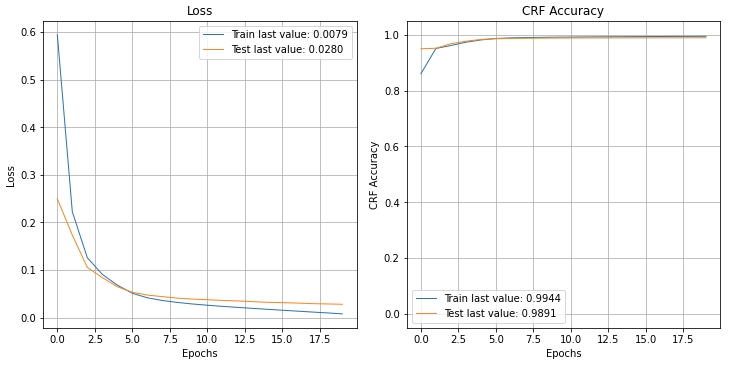
The performance is not bad, generally approaching 99%, but it can definitely be higher with hyper parameter tuning (i.e. the dimension of the LSTM states, the embedding, using pretrain embedding).

Further this 99% accuracy does not tell the full picture because we should look at the individual class performance (i.e. how does the model predict on B-org vs B-per?). To do this, we can plot the multi-class confusion matrix.

y_pred = ner_model.predict(X_test)
y_pred_dense = np.argmax(y_pred, axis=2)
y_test_dense = np.argmax(y_test, axis=2)

# First arg is true label, second arg is for prediction
# Result in a confusion matrix where each row represents a different true label
# and each column represents a different prediction
cm = confusion_matrix(y_test_dense.flatten(), y_pred_dense.flatten())
plt.figure(figsize = (12,12))

tags = [index2tag[i] for i in range(num_tags)]
ax = sn.heatmap(cm+0.001, annot=False, square=True, norm=LogNorm(), xticklabels=tags, yticklabels=tags)
ax.set_title('Confusion Matrix of NER Tags')
ax.set_xlabel('Prediction')
ax.set_ylabel('Ground truth')

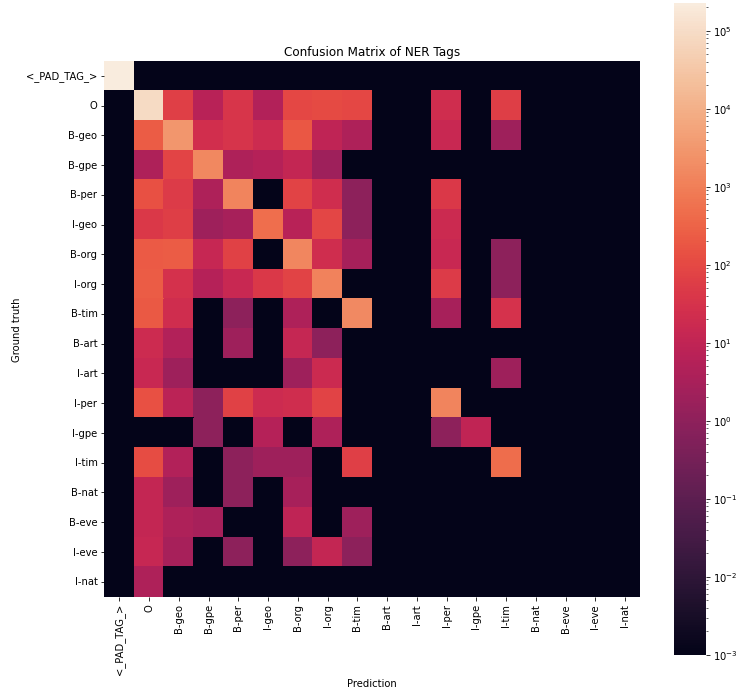
The confusion matrix is ploted using a heatmap in log scale. I had to use log scale because the dataset is dominated by the padding and O tags, which are not as interesting. A couple problem we can notice on the graph is that B-art, I-art, B-nat, B-eve, I-eve, I-nat columns are all black, which means our model did not predict these POS tags. This can be a problem. Let’s dig into them further by plotting the individual 1-vs-all accuracy, precision and recall (see Advanced Classification Metrics: Precision, Recall, and more)

cm2 = multilabel_confusion_matrix(y_test_dense.flatten(), y_pred_dense.flatten())
result = []
for i in range(num_tags):
  tag = index2tag[i]
  # get the 2x2 confusion matrix for a particular tag
  # [ true-neg,   false-pos]
  # [ false-neg,  true-pos]
  cm2b2 = cm2[i]
  result.append({
      "Tag": tag,
      "Accuracy": (cm2b2[0,0]+cm2b2[1,1])/np.sum(cm2b2),
      "Precision": cm2b2[1,1]/(cm2b2[0,1]+cm2b2[1,1]),
      "Recall": cm2b2[1,1]/(cm2b2[1,0]+cm2b2[1,1]),
  })
metrics_df = pd.DataFrame(result)
metrics_df

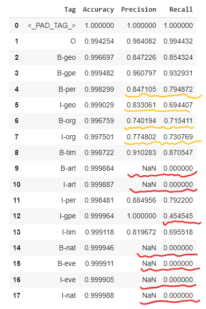
From the table, we can see a few problems

• Recall is 0. This agrees with our previous findings that our model is biased and does not produce any prediction for some of the tags.
• The NaN precision value is due to a divide by 0 problem because precision = True Positive / (TP+FP). (see Advanced Classification Metrics: Precision, Recall, and more)
• Precision and recall is much worse than accuracy for B-per, I-geo, B-org, I-org. This is a problem of the imbalance of our data. It’s much easier for the model to predict the popular tags to achieve high accuracy and just ignore the rare tags.

Besides hyper-parameter tuning, some other thigns we can try includes:

• Using a larger data set
• Get more balance data for rare labels
• Using a pretrained word embedding

Appendix (CRF layer)

The CRF layer models the conditional probability between adjacent tags, and the objective function is define as below:

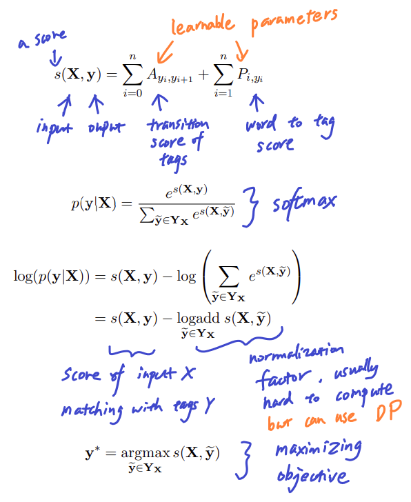
If you dont’ understand all these, it’s okay. The main point to know is tha the CRF layer gives a way to optimize (1) transition score between tags and (2) word to tag score, so that the probability of a given input word representation (x) and output tags (y) can be be maximized.