Solving MDPs with dynamic programming

In Reinforcement Learning, one way to solve finite MDPs is to use dynamic programming.

Policy Evaluation (of the value functions)

It refers to the iterative computation of the state-value functions for a given policy (using k to get to k+1)

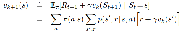
As k goes to infinity, the value function v should converge to the value function for the given policy. This algorithm is called iterative policy evaluation.

Each step of the operation above is called expected update.

This method of evaluating the state-value function using the previous version is a form of bootstrapping.

To fully evaluate a policy, you need to sweep over all state s in the state space (which can be done synchronously or asynchronously).

Policy Improvement

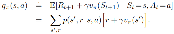
With policy evaluation above, we can obtain the associated state-value function, but we still need to get the best policy. Policy improve refers to the computation of an improved policy given the value function for that policy.

One way to check if the existing policy is good for state s is by taking another action a for the current step and thereafter following the existing policy again.

If this is better, would it be even better to just follow action a thereafter every time? The Policy Improvement Theorem states that this is true!

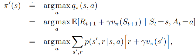
This can be applied to all states and all possible actions in general as well. So for every states, we constantly look for the best action a that maximized the return of this one-step greedy action.

The associated policy can be expressed as pi-prime

If we get to a point where pi-prime is no better (no improvement) over pi, we know the state-value function of pi and pi-prime at the same.

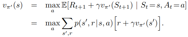
This is the same equation as the Bellman optimality equation! So this state-value function must be v*.

In another word, if a policy is greedy with respect to its own state-value function, then it is an optimal policy.

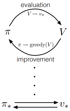
Policy iteration: two most popular dynamic programming methods

• Policy iteration: for a finite MDP, we can alternate policy evaluation and policy improvement to converge to the optimal policy and value functions.
  • Policy evaluation could be slow since it may require multiple sweeps of the state space to converge to a state-value function.
  • Many sweeps of policy evaluation for each sweep of policy improvement
• Value iteration: get be faster
  • Truncate the policy evaluation early
    • Just run one sweep of the state space for policy evaluation
    • Optimize the action a with this one-step sweep value function
    • 
    • This does not get to the final state-value function in one step because the it is still using an imperfect state-function v_k
    • Next we come back to policy evaluation again with just one sweep.
  • One sweep of policy evaluation for each sweep of policy improvement
  • In practice, value iteration has faster convergence than policy iteration. (I see some similarity with stochastic gradient descent vs batch gradient descent in deep learning)

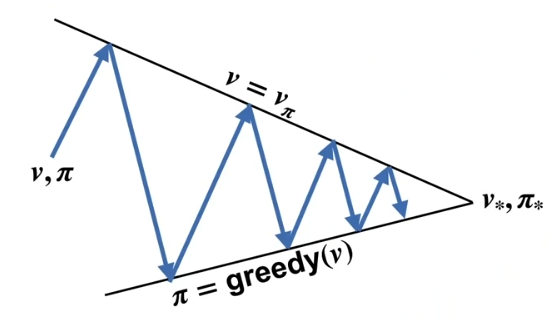
Generalized policy iteration (GPI)

• The policy iteration and value iteration methods are types of generalized policy iteration.
• Policy evaluation and policy improvement processes can interleave in its own independent granularity
• Policy keep improving each time and value functions keep approaching the value function of the policy
• When the policy and value functions stabilize, they must be optimal (consistent with the Bellman optimality equation)
• Value iteration above is a type of GPI.

Conceptually the classical policy iteration is alternating between policy evaluation and greedily search the action

In fact we don’t even need to fully evaluate the policy or fully greedify the action at each step.

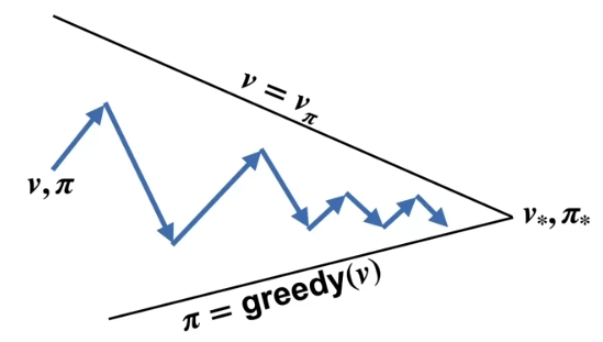
This can achieve quick converging in time.

Efficiency of dynamic programming

• DP is not very efficient (has polynomial run time over the state and action space)
• Curse of dimensionality: the size of the state space grows exponentially as the number of features. But this is rather a nature of the problem, not an issue of dynamic programming.
• DP is still better than direct brute search, which has exponential run time pow(|Action|, |State|) because every state has |Action| actions to choose from.
• DP scales better than linear programming (LP will be impractical at smaller number of state and action space)
• Even in case the number of states is too large, DP can still solve problem sometimes when the state space along the optimal trajectories is relatively small
• Asynchronous DP is needed for large state space usually (need to ensure all states are visited all the time)

Final note

Is dynamic programming the solution to reinforcement learning?

• Dynamic programming relies on knowing the model of the MDP (dynamic of the environment), but this is often not known in practice.
• Dynamic programming does not interact with the environment
• Dynamic programming solves MDP but not necessarily reinforcement learning problems.
• Most reinforcement learning algorithms are approximation of the dynamic programming algorithm

Reference: most of the material of this post comes from the book Reinforcement Learning