Planning with Tabular Methods in Reinforcement Learning

Tabular methods

Tabular methods refer to problems in which the state and actions spaces are small enough for approximate value functions to be represented as arrays and tables.

Two types of RL methods

There are two type of reinforcement learning methods:

• Model based: methods that require a model of the environment
  • Dynamic Programming
  • Heuristic search
• Model free: methods without need a model of the environment
  • Monte Carlo method
  • Temporal difference method

Two types of models

• Sampling model
  • More compact (require less memory)
  • Compute probability by averaging samples
  • Ex: rolling a single die 12 times
• Distribution model
  • Modeling the distribution in the sample space
  • Explicit: Can compute exact probability
  • Ex: modeling the joint distribution of 12 dice (power(6, 12) outcomes)

Planning in RL

Planning the process of producing (or improving) a policy from a model

Two types of planning:

• State-space planning: search through the state space for an optimal policy or an optimal path to a goal
• Plan-space planning: search through space of plans (skipping this for now)

Connection of planning to Q-learning

• Q-learning uses experience to update a policy
• Q-planning uses a sample model to update a policy

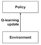vs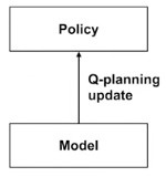

One type of Q-planning

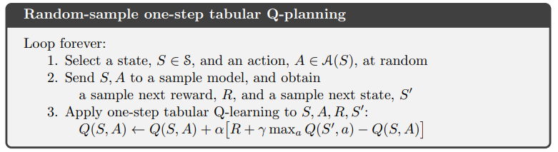
• Sample a trajectory using the model
• Use Q-learning to learn Q(s, a) with greedy selection
• Improve policy with greedy action

Dyna Architecture

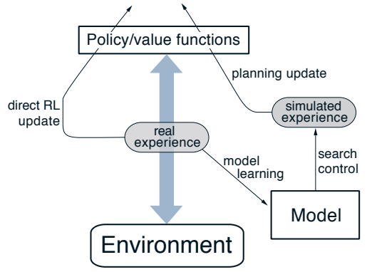
• Update the action-state function using Q-learning
• Also update the model on the environment by learning about the environment at each time step
• Perform planning when there is a model that can be used to search for a policy from certain state

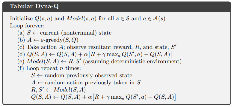
• The first 4 steps are the same as Q-learning (direct RL)
• Step e update the model dynamic
• Step f (indirect RL)
  • n is the number of planning steps to run
  • each time, pick a random but previously seen state-action pair
  • use the model to generate the next state and reward
  • perform the same Q-learning update step again
• The planning process is most compute intensive
  • At the beginning, most of the return could be zero and update is slow, but once the return start propagating to more state, it will speed up significantly
  • It’s much faster than Q-learning RL because it has many more chances to update Q(s,a) during planning.

Inaccurate Model

The performance of planning process in the algorithm can depend on the model accuracy. What if the transition probabilities stored in the model is not accurate?

• Incomplete model: at the beginning, the agent has not visited all the states
  • Dyna-Q makes sure to only sample from previously seen states, so it will only update those the state-action value function for these state-action pairs.
• Environment changes: stored probabilities and reward no long reflect reality
  • This might cause the state-action value function Q to move in the wrong direction
  • Want to revisit or double check a state that has not been visited for a long time

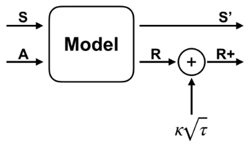
Dyna-Q+

A reward is added to each state by kappa * sqrt(tau)

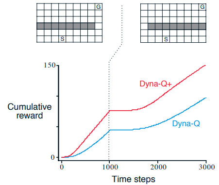
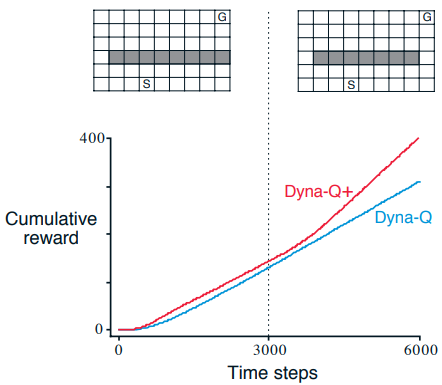
Examples

Dyna-Q+ can find the new solution quickly when the environment becomes harder

Or when the environment becomes easier. It might take a long time for Dyna-Q to discover the new solution by exploring slowly with epsilon probability.

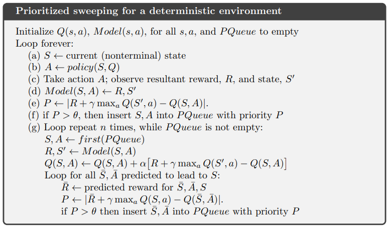
Prioritized Sweeping

In regular Dyna agent simulation, it’s more efficient to if simulated transitions and updates are focused on particular state–action pairs.

• Backward focusing: work backward from arbitrary states that have changed in value, either performing useful updates or terminating the propagation
• Prioritized sweeping:
  • A queue is maintained of every state–action pair whose estimated value would change nontrivially if updated , prioritized by the size of the change
  • When the top pair in the queue is updated, the effect on each of its predecessor pairs is computed.
  • If the effect is greater than some small threshold, then the pair is inserted in the queue
    with the new priority (if there is a previous entry of the pair in the queue, then insertion
    results in only the higher priority entry remaining in the queue).

In an stochastic environment, we use expected update, which can be slower than sampling update.

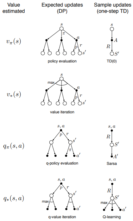
As a recap here is all the one-step update with 8 combinations

• Whether state value function v or state-action q value function is learned
• Whether expected updates (DP) or sample updates (one-step TD)
• Whether it’s on policy (v_pi or q_pi) or off policy learning (v* or q*)

Reference: most of the material of this post comes from the book Reinforcement Learning