Finite Markov Decision Processes (MDP)

Finite MDP is the formal problem definition that we try to solve in most of the reinforcement learning problem.

Definition

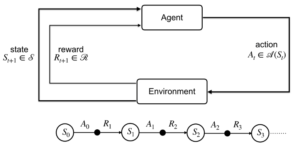
Finite MDP is a classical formalization of sequential decision making, where actions influence not just immediate rewards, but also subsequent situations, or states, and through those future rewards.

Compared to the multi-armed bandit problem, the expected reward q function is different

• Bandit problem: q*(a)
• MDP: q*(a, s) where s is the state
  • v*(s) is the value associated with the optimal action selection for state s

The MDP sequence trajectory: S0, A0, R1, S1, A1, R2, S2, A2, … (note the subscript for time, there is no R0)

Dynamics of MDP is completely defined by the function:

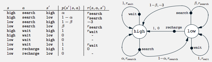
Transition Graph of a can collecting robot

Suppose we have a robot that collects cans from the office. It can search, wait, and recharge.

We can model the full state transition using this function p.

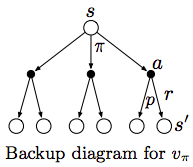
• The white big nodes are “state nodes”
• The black solid nodes are “action nodes”
• The arrow represents a transition after taking an action with probability and reward

Reward Hypothesis

Purpose of the agent is to maximize the expected value of the cumulative sum of a received scalar signal (called reward).

• Note that this reward signal is different from the immediate reward specified in the transition graph above.
• This hypothesis states the importance of the reward signal in guiding the agent to optimize its behavior to achieve the final goal.

This hypothesis has some challenges in guide the behavior in some situations below

• Representing risk since expected value is used
• Encouraging diversity behavior (don’t want to recommend the same song over and over)

Episodes

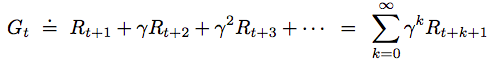
The agent tries to maximize the total reward as follow:

where T is the final step. T is where we can break the sequences into subsequence where it ends in a special terminal state, followed by a reset.

• Wining or losing a chess game is an episode
• Each episode is independent from how the previous episode ended
• A task with episodes of this kind is called an episodic task.

In contrast, the agent–environment interaction does not break naturally into identifiable episodes, but goes on continually without limit. We call these continuing tasks. Since reward would be infinite for an continuing task, we introduce discounting to the total reward:

It can also be expressed in recursive form:

Policy and value functions

• The policy is denoted as action given state
  • 
  • Can be deterministic or stochastic
• Value functions: return the expected total reward in the rest of the game
  • The state-value function is specified as the total reward with starting state s and following a policy pi thereafter
    • 
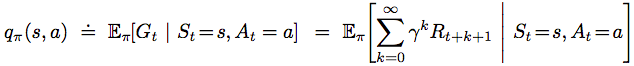
  • The action-value function is the value of taking action a starting at state s and following policy pi thereafter
    • 

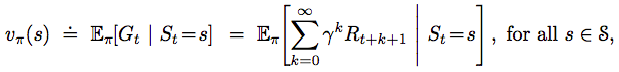
Both value functions above can be estimated by Monte Carlo methods because they involve averaging over many random samples of actual returns.

Bellman equation for state-value function

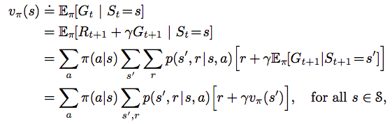
It defines the state-value function recursively using all the successor states. The two summations can be represented by the two layers of the Backup diagram below

Similar, it can also be done for the action-value function q*

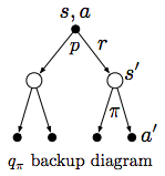
But normally, we can just calculate q (action-value function) from the the state-value function (don’t need to go two layers deep).

Solving the Bellman equations is basically solving a system of linear equations that is otherwise hard to solve with an unmanageable number of states. Still for some problem, the number of state-value equations would be intractable many that it’s not possible to solve the Bellman equation (ie Chess)

Optimal policy

We can find the optimal policy that

• maximizes the state-value function for a given state s
• maximizes the action-value function for a given state s and action a

It’s possible to solve for the Bellman equation for small problem. But in practice, most problem are quite large in the state space that we can only rely on compact parameterized approximated representation.

Solving Bellman Optimality Equation

Searching for the solution of the Bellman Equation is basically solving a system of linear equations, but that does not help us find the optimal policy (we can only brute-force to iterate over all possible policy and solve the Bellman equation to find the solution). A better way is to use the Bellman optimal equations below:

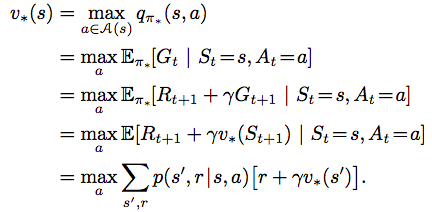
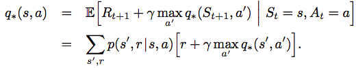
Note that here both value functions do not depend on the policy. Instead a “max over a” operation is used. There are various techniques to solve for v*(s). From v*(s), we can easily solve for q*(s,a) and the optimal policy.

Reference: most of the material of this post comes from the book Reinforcement Learning