Multi-Armed Bandit Problem

Pre-requisite: some understanding of reinforcement learning. If not, you can start from Reinforcement Learning Primer

Goal

Let’s analyze this in the classic Multi-Armed Bandit problem using the epsilon-greedy strategy.

Set up the experiment

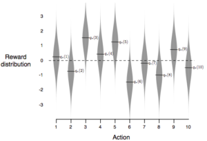
We can set up an experiment as follows

• K=10 for 10-armed bandit (with 10 actions to choose from)
• Each arm has a Gaussian distributed return (with some mean and standard deviation of 1)
• The mean of each arm is randomly initialized using the standard Gaussian distribution (mean=0, variance=1)
• Repeat this simulation many times by regenerating the 10-armed bandit each time

The epsilon-greedy strategy

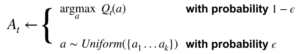
• Select the best action under Q with probability 1-epsilon
• During the small probability epsilon, selection randomly among all possible actions with equal probability
• We want to analyze the reward of the agent from t=0 to steady state
• Q is estimated using sample average method (step size = 1/N(a)) where a is the action at time t

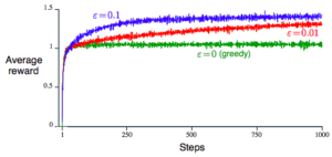
By running experiment 2000 times for different values of epsilon and average the reward at each time step, we get an average reward plot like below

Notable observation about the strategy

• There is an optimal epsilon
  • Greedy (epsilon = 0) is not good because agent might be wrong in choose the best paying arm
  • Large epsilon is also not good, because spending time exploring
• The optimal epsilon
  • depends on the variance of each bandit
    • If variance is 0, then greedy approach is optimal
  • depends on the prior distribution that we use to generate the mean of each bandit
    • But this is usually unknown in practice, and even knowing it does not help to be optimal in a specific bandit problem
  • depends on the time horizon we look at
    • if we instead look at 10000 steps, small epsilon will perform better because it would have more time to explore before plateau
• The mean of each bandit does not change in a given bandit problem. This means the problem is stationary
  • In practice, the mean of a bandit could change over time (non-stationary)

Step size (alpha)

The step size can also play a role in the performance. In the above setting, the step size is set to be 1/N(a), but it can be generically represented as alpha below

• Large alpha: Q quick catches up to q* but it will oscillate due to the randomness of the new sample (too much over correction)
• Small alpha: takes a long time for Q to catch up to q*
• N(a): able to quick move to estimate q* and then stabilized and converge to a steady state
  • However N(a) is good for stationary q* only, we will learn later that larger alpha with over correction can be beneficial for Q to adapt dynamically to a changing q*

Optimistic initial value

There is also another way to impact the exploration behavior by giving some high value for Q1. This makes the agent more like to explore the unexplored and be “disappointed” a few times before realizing its not a good object. It can even help a greed algorithm to perform better.

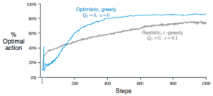
However, this is not good enough because it only encourages exploration in the beginning. If the environment is not stationary, then the greedy approach will be stuck at the old optimum. It’s also hard to know what is a good initial optimistic value in prior.

Upper Confidence Bound (UCB) Action Selection

To better balance the exploration and exploitation, we can use the confidence bound to make decision on the action. In comparison to the epsilon-greedy approach:

• epsilon-greedy: based on expected reward
• UCB: based on a confidence upper bound

In particular, we choose by the action that has the best upper bound below which is action 1:

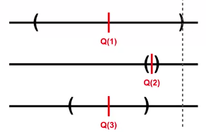
This is formulated as

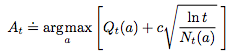
where

• c is the tunable parameter for the confidence. It’s a hyper-parameter that balance exploration and exploitation.
• t is the current time – the higher the larger the upper bound
• Nt(a) is the number of times that action a has been selected

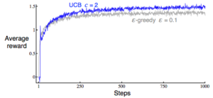
We see that UCB with c=2 can beat the epsilon-greedy strategy in the long run.

Real world RL

While the multi-armed bandit problem seems quite simple, it’s the primary way that Reinforcement Learning is currently applied in the real world. One of the challenge is the need to use a simulator for the agent to interact with and learn.

The general guideline is a paradigm shift to make RL work in the real world.

• Better generalization
• Let the environment take control
• Focus on statistical efficiency
• Use feature to represent the state
• Algorithm should produce evaluation in the process of learning
• Look at all the policy (the trajectory of policy) rather than just the last policy in a simulator environment

Limitation of this model

The multi-armed bandit does not model all aspects of a real problem due to some limitations

• There is always a single best action independent of the situation. That is, you don’t need to make different action based on the situation
• The reward is not delayed. You get the reward in one step. Each episode is just one time step.

The Markov Decision Process (MDP) provides a richer representation.

Contextual bandit

The contextual bandit (aka associated search) algorithm is an extension of the multi-armed bandit approach where we factor in the customer’s environment, or context, when choosing a bandit. For an example of personalized new recommendation, a principled approach in which a learning algorithm sequentially selects articles to serve users based on contextual information about the users and articles, while simultaneously adapting its article-selection strategy based on user-click feedback to maximize total user clicks.

Reference: most of the material of this post comes from the book Reinforcement Learning