Practical Intuition of the Gaussian Process Regression

When I first learned about the Gaussian Process (GP), I have a hard time getting the intuition about it.

From Wikipedia, the definition of GP is

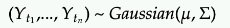
A time continuous stochastic process is Gaussian if and only if for every finite set of indices in the index set

is a multivariate Gaussian random variable. That is the same as saying every linear combination of has a univariate normal (or Gaussian) distribution.

While this definition is elegant, I find it hard to understand and to apply to ML model like Gaussian Process Regression (GPR). So the goal of this post is to provide some intuition to understand GP for practical purpose.

Definition of GP (again):

You can pick n indices from the process to generate n random variables, and these n variables are distributed according to a joint Gaussian.

I decide to use Y instead X for the label of the data because I want to reserve X for the features of the data.

So where is X (feature variables) in the distribution above?

The mean (mu) and covariance matrix (sigma) are both functions of x.

• But often the mean is just 0 (constant) and is uninteresting
• The covariance matrix is defined by a kernel function, which is the most interesting part of GP

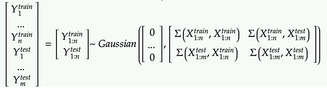
In fact, the prior of the distribution of Y is as follow:

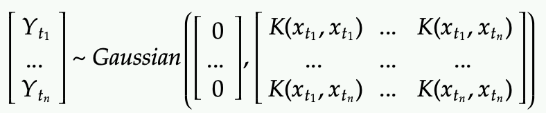
• There are n random variables Y that are chosen.
• These n Y variables at different indices are distributed as joint Gaussian with mean 0 and covariance matrix defined by the Kernel function
• The covariance between a pair of Y’s at indices i and j are controlled but the kernel function evaluated by the corresponding x at indices i and j.

One common Kernel function is the RBF:

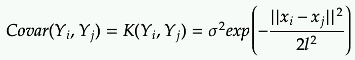
You can interpret this kernel as follow:

• It gives the covariance between any pair of Y at indices  i and j based on their features (X) at indices  i and j.
• This RBF kernel outputs
  • large value (close to 1) when the features are close to each other at indices i and j
  • small value (close to 0) when the features are far from each other at indices i and j

Apply the GP to Gaussian Process Regression (GPR)

First, define the data set with training data (size n) and testing data (size m):

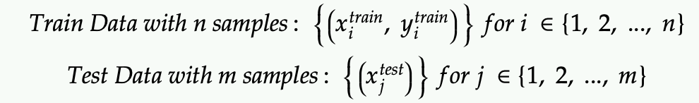
Note that in the test data set we don’t have the test label because that’s what we are trying to predict.

Second, rewrite the prior of Y with the train and test data split:

Next we want to substitute the 4 blocks of covariance matrices with the kernel function.

• Each of them is essential the kernel matrix
• So far we have assume that Y train might have perfect measurements and this is not realistic. One option is model some noise in the measure of Y train.

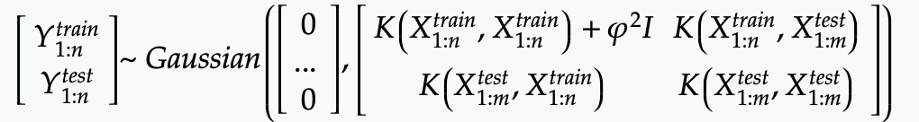
Note that we only add some noise with variance phi-squared for Y_train (phi is another hyper parameter to be tuned to control how confident we are around the measured data in Y train)

We are now finally ready to apply some Bayesian Inference (ie getting the posterior distribution).

Basically we want to get the PDF of Y test. Since we model Y test as another Gaussian distribution, this is equivalent to finding its mean and covariance matrix.

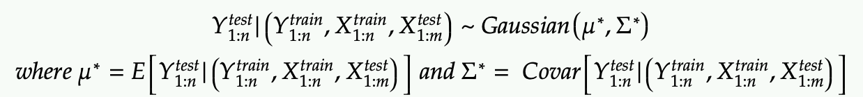
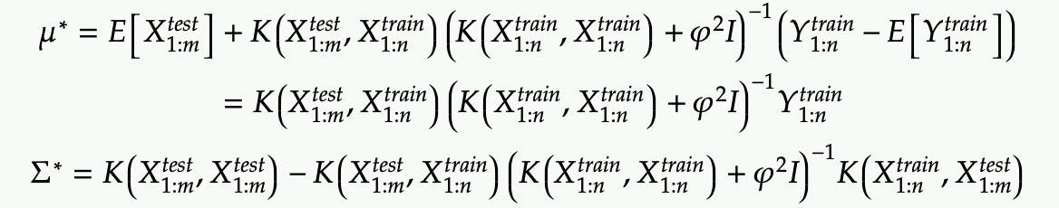
This is a direct application of Gaussian conditional probability (with block matrix inverse)

Again if the above result is not clear, I suggest you to read my other post on conditioning Gaussian distribution

Takeaways

• The mu start from above is the mean of the prediction using Gaussian process, while the sigma start provided the variance of each test data point (along the diagonal of sigma star).
• The take home intuition is that we have related all the Y train and test via multivariate Gaussian, which allows us to apply conditional distribution on the Y test given Y train.
• The significance of GP is that it not only returns the expected prediction but also a confidence (via variance) of the prediction.

Where is the parameter training step?

The GPR model is a lazy model, which means it does not require any training, or that it does the training and inferencing in one step (sort of like Near Neighbor Model). As you can see the mu and sigma are calculated in one step with all the training and test data.

The GPR model is also non-parametric. This means it does not have coefficients like the linear regression. All the knowledge of the model is basically contained in these Kernel matrices which depends on the size of the data set. The matrices are of size O(n^2) which mean inverting these matrices are not so efficient when n is large.

About hyper parameters

3 hyper parameters are used in the GPR

• The RBF kernel has a l value that controls how far are the features allowed to be away to be still causing a correlation between their corresponding labels.
  • The smaller it is, the most it trusts the local value and causes the curve to be more wiggly.
• The RBF kernel has a lower-case sigma value that controls the total variance (amplitude)
  • The large it is, the larger the predicted confident interval (ie the spread of the band) in the result
• The prior distribution has a phi value that controls our belief in the observed value of y train
  • The smaller it is, the more confident we are about the observed values. This forces the model to generate a curve to pass the training point more exactly.

You really need to tune the parameters to get the desirable effect.

About the kernels

RBF

• We use the RBF kernel because it’s most commonly used.
• It’s called “exponentiated quadratic kernel” or “radial basis function” or “squared exponential kernel”

There are other interesting kernels

• Matern kernel – another stationary kernel that give additional parameter to control the smoothness
• Periodic kernel – with a sinusoidal term to model repeated patterns.

Additional resource

Check out this website for some interactive tool to play around with the parameters of GP: link