The multi-armed bandit problem is a very interesting problem in statistics. This post will use this scenario to explain two topics:
- Beta Distribution
- Thompson Sampling (at the end)
Beta Distribution
The Beta distribution is a continuous distribution for a positive random variable (X). It has two parameter alpha and beta that controls the shape of distribution. The best example to understand it is by modeling the bias of a coin given evidence of the coin flips.
Scenario:
- There is a coin that has a probability p of flipping head and (1-p) of flipping tail.
- We are able to observe some number of flips of this coin.
- h: number of heads
- t: number of tails
- What can be deduced about the value of p after the observation?
We can first write out the likelihood of an event with h heads and t tails
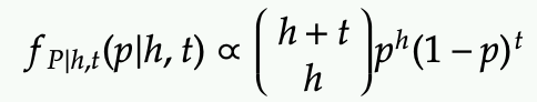
- This looks like the binomial distribution but it’s different because the variable is p here (in the binomial distribution, p is a parameter).
- The proportional sign is used instead of equality because the coefficient does not depend on p and is not important (will be normalized later).
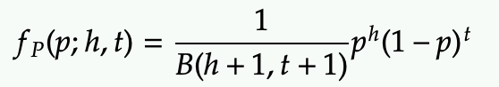
If we want to turn the above likelihood into a probability (PDF) over P, we can integrate p over [0,1] to find out the area underneath so that we can use that area as a normalization factor.
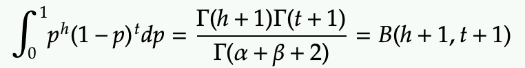
The normalization factor is a constant (independent from p).
- It can be expressed by a few Gamma functions, which are same as factorial when alpha and beta are natural numbers.
- It can also be expressed by the Beta function, which is used for the coefficient of the Beta distribution.
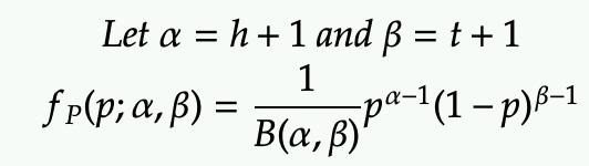
However the above for expressed in h and t are not the standard form that is commonly use. Instead, we use parameters alpha and beta:
- alpha = h + 1
- beta = t + 1
Let’s example some sample plots:
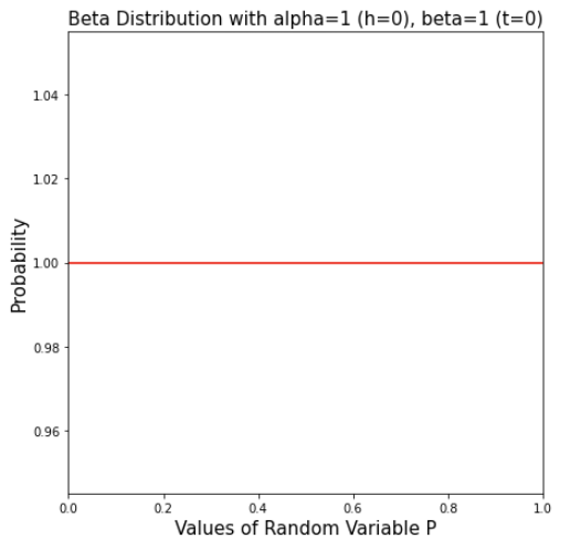
1) No evidence (heads=0, tails=0)
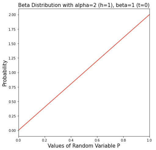
2) Only one head
Note that the pdf is highest near p=1 and lowest near p=0, suggesting the model believes that p is more likely to be near 1 (more biased to head)
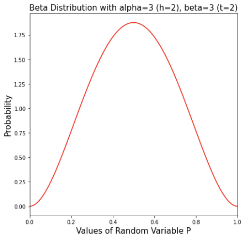
3) 2 heads and 2 tails
Note that peak value of p is at 0.5, which matches the observed probability of 2/(2+2)=50%.
The probability of at the two extremes (p=0 or p=1) is at 0, which means there is no way that p=0 or p=1.
The spread of the curve is quite “fat”, which means already we believe the maximum likelihood is 50% but it’s not quite certain given the evidence (ie. it could be 0.4 or 0.6 at similar likelihood).
4) 29 heads and 29 tails
This pdf has the same peak at p=0.5, but the spread is much more narrow. Also the peak is much high (note the scale on the y-axis).
With more evidence (more flips), the model is more confident in the value of p near around 0.5.
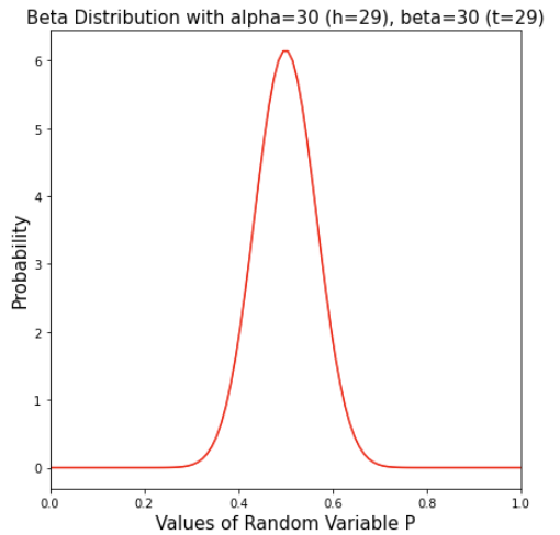
Now the Beta distribution is starting to look like a normal distribution.
Note that I have only covered the case when alpha and beta are natural numbers. It’s possible to apply the Beta distribution with alpha>0 and beta>0 on non-integer values. I have not developed a good intuition around that yet, so I will skip that part.
Thompson Sampling
Thompson Sampling a way to apply the Beta distribution to the multi-armed bandit problem.
Scenario:
- A player is facing row of slot machines in a casino.
- In each round, the player can choose to play at one of the slot machines.
- The player either win $1 or not ($0) each time at the slot machine that he is playing.
- The player want to maximize the payout by playing these slot machines
- Each slot machine has an internal parameter p that decides it’s probability of winning in each round (p is specific to each machine and is constant)
Strategy:
- Explore: want to find out the best machine, which is the machine with the highest p value
- Exploit: want to play as often as possible as the best machine
Question: how do you balance between playing at the “best” machine so far (the one that has the high winning probability from your observation) vs spending more time to play at other machine that might be an even “better” machine.
Example:
Let’s you have been playing for a while among 3 machines
- Machine 1: won 3 times, lose 7 times (observed p=0.3)
- Machine 2: won 0 times, lose 1 times (observed p=0.1)
- Machine 3: won 7 times, lose 3 times (observed p=0.7)
Greedy strategy (exploit only):
You always choose Machine 2 to play because it has the highest p from your observation so far
The problem of this strategy is that you will never play at machine 2 any more but it might have a high p but you got unlock the first time and you lost.
Conservative strategy (explore a lot):
You keep playing among all 3 machine machine regardless of their current observed win rate. For example, you just play at least 100 round of each machine. You might arrive at some result such as below
- Machine 1: won 32 times, lose 68 times (observed p=0.32)
- Machine 2: won 80 times, lose 20 times (observed p=0.8)
- Machine 3: won 55 times, lose 45 times (observed p=0.55)
After the 300 rounds, you feel that you have a pretty confident measurement of each machine, then you decide that machine 2 is the best machine so you keep playing machine 2 afterward.
The problem of this strategy is that you spend a lot of time exploring the bad machines (ie machine 1) which had low payout. What if the Casino shuts down after you play 300 rounds.
Thompson Sampling: choose the machine based on its distribution of p
For each machine, we collect its history of winnings and losses. This gives us a probability distribution of its p by the Beta PDF.
- Machine 1: won 3 times, lose 7 times (observed p=0.3) => Beta(alpha=3+1, beta=7+1)=Beta(4, 8)
- Machine 2: won 0 times, lose 1 times (observed p=0.1) => Beta(1, 2)
- Machine 3: won 7 times, lose 3 times (observed p=0.7) => Beta(8, 4)
Next we sample from each of the Beta distribution, so we generate 3 values.
Based on the highest value, we choose the associated machine to play.
After we play, we add the win/loss to the evidence again and keep repeating this process.
The Thompson Sampling strategy provides a balance between exploration and exploitation.
- Each machine get a chance to be play (because of the sampling nature on its P distribution returning a value between 0 and 1
- The machine with “better” winning history gets chosen more often.
- The machine with “worst” winning history gets chosen less often.
- The machine with “lower” evidence get wider spread in its Beta distribution, and thus has more volatile values. So even a machine with low win rate (0 win, 1 loss => 0% win rate) can get chosen between the its sample value of p can still be large.
Is it an optimal strategy?
Unfortunately, the answer is more complicated. Proving whether Thompson Sampling is the optimal strategy is a bit beyond the scope of this post, but the short answer is that it is optimal in some general reinforcement learning (RL) environment asymptotically.