This tutorial introduces the Poison Process, and will give an quick tutorial to understanding 3 related distributions
- Exponential Distribution
- Poisson Distribution
- Gamma Distribution
Exponential Distribution
We should first talk about the exponential distribution first to lay some ground work before going into the Poisson process
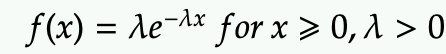
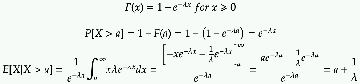
The PDF of the exponential distribution is given by
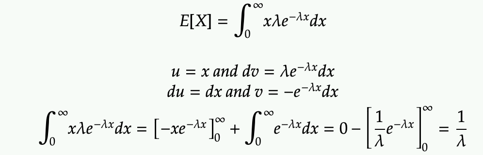
The mean of a exponential variable is 1/lambda:
The CDF can be easier derived from PDF by integration:
![]()
One important property of the exponential distribution is the memoryless property.
In the plot below
- The black curve the Exponential distribution, and the area under the black curve is 1 (from 0 to infinite on the x-axis)
- The area under the blue curve is P(X>a)
- Note that the blue curve has the same shape as the black curve
- The red curve is the same as the blue curve, but rescale to have the area under the red curve to be 1
- Now observe that red curve is basically the black curve shift to the right by a
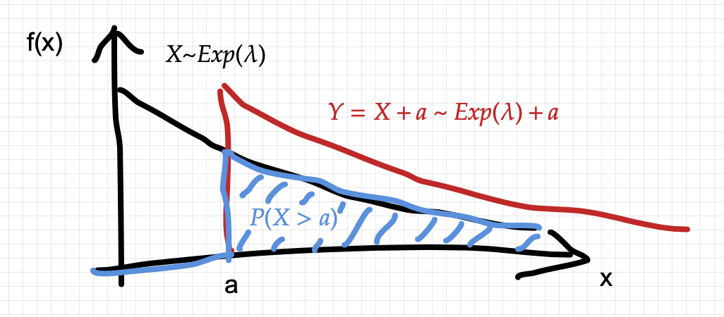
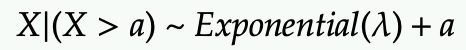
So the expected value of X given X > a is just adding a on top (for a>=0). We can verify it with some direct evaluation of the expected value with integration again:
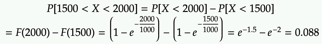
Example Problem:
Let X be the life of a light bulb, and we model X as an exponential distribution:
- The average life of a light bulb is 1000 days
- What is the probability that the light bulb will die between 1500 and 2000 days?
, then we have E[X]=1/lambda=1000, so lambda=1/1000.
X ~ Exponential(lambda=1/1000)
This distribution allows us to answer a question like
Poisson Process
The poisson process defines a series of discrete events where
- The time between events is exponential distributed with known lambda parameter
- Each event is random (independent of the event before or after)
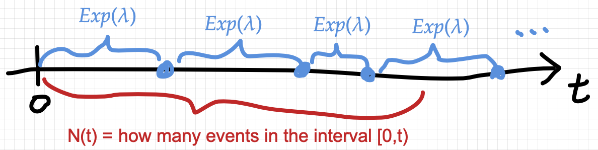
We can define a count process {N(t), t>=0} with the number of event of event occurrence during a time interval t.
Then N(t) follow a Poisson distribution (PMF – probability mass function) given by:
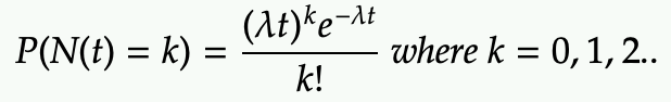
The rate parameter lambda is defined to be number of event per unit of time. It also models the inter-arrival time with Exponential distribution with the same parameter lambda.
Example problem:
Scenario: Count the number of bus arrival at a bus station where the inter-arrival time is model by Exponential distribution.
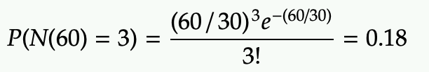
Question: If the mean arrival time is 30 minutes, what is the probability that exactly 3 buses arrive in 60 minutes?
First, we calculate the rate parameter r using the mean arrival time. So r = 1/30 (unit is arrivals/minute).
Next, we apply the formula with r=1/30, t=60, k=3:
The Poison distribution is quite useful and interesting, but it focuses on the number of event occurrences in some time interval in a Poisson Process. Just think of them as two ways of looking at the problem.
Gamma Distribution
Let now motivate some discussion on the Poisson Process to (eventually) lead to Gamma distribution (please be patient :D).
Question1: current time is t=0, what is the expected arrival time of the next bus?
Answer:
- It is given that the inter-arrival time is Exponential distribution with parameter lambda.
- The expected value is 1/lambda.
- This is an easy application of the exponential distribution
Question2: current time is t=0, what is the PDF of the arrival time of the 2nd bus?
Naturally, we want to just add up the two inter-arrival times
- Let X1 be Exp(lambda)
- Let X2 be Exp(lambda)
- X1 and X2 are independent.
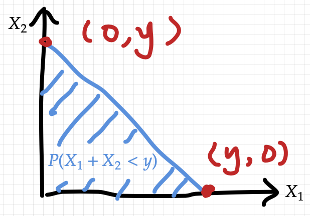
- We want Y=X1+X2
Method 1)
We can start by getting the CDF of Y (ie. P(Y<y)) by integrating the 2D PDF over the blue triangle below:
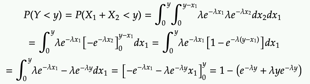
The PDF can be derived by differentiating the CDF

Method 2)
We can use the Poison distribution to derive the CDF of Y
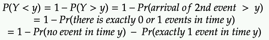
It takes a bit of thinking to get the logic straight on above derivation
- If we want the 2nd arrival to be after time y, then there 2 situations can happen during time y:
- No event occurs, this mean even the first event is after time y
- Only 1 event occurs, so second event must be after time y
- Since the two situation are mutually exclusive above, we can just break them up separately.
Next we define Z to be the Poison random variable that models the number of events in time y.
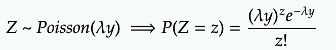
So we can rewrite P(Y<y) with the help of Z

Note that the resulting CDF is the same as method 1.
Generalizing to Gamma Distribution
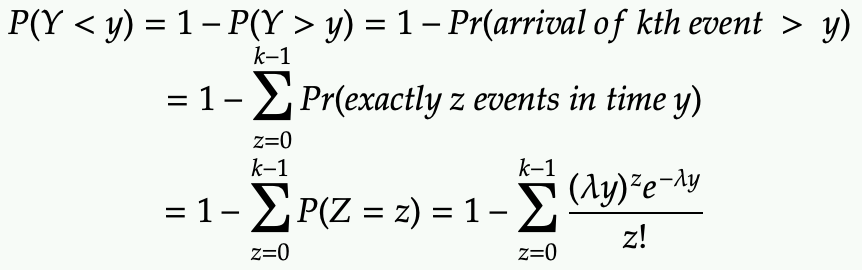
While method 1 and method 2 give the same result, method 2 is actually a bit easier to generalize for k-th arrival.
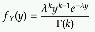
The probability distribution of the k-th arrival is precisely the Gamma distribution!
We can first write the CDF of the Gamma distribution of k-th arrival as below:
Next we can differentiate the CDF to get the PDF
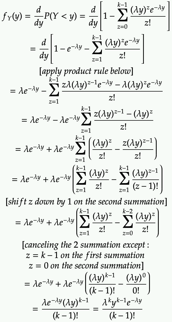
Technically, what we are derivate is the Erlang distribution, the Gamma distribution reflex the assumption on k from just integer to any positive real number.
In wikipedia, the formula uses alpha and beta as the parameters
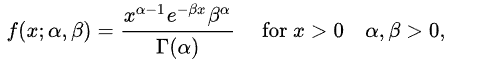
- alpha (k) is called the “shape parameter”
- The Gamma distribution becomes a Exponential distribution when alpha=1
- The larger it is, it moves the peak of the PDF further to the right.
- It affect the curvature of the PDF (how it goes up and down)
- beta (1/lambda) is called the “rate parameter” or “scale parameter”
- When beta is larger (lambda is smaller), it stretches the entire curve to the right
- It maintains the curvature of the PDF
“Shape parameter” is a very bad name because changing either parameter technically modifies the shape, but let’s explore some graph to understand the Gamma distribution.
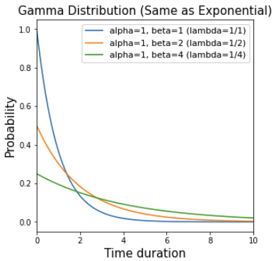
1) Alpha=1, varying beta (1/lambda)
The effect of changing beta is really the same as changing the lambda of an Exponential distribution.
Note that the 3 curves are just different version of the horizontally stretched PDF with normalization to maintain area-under-curve (AUC) to be 1.
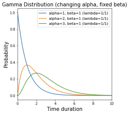
2) Varying alpha, fixed beta
The effect of varying alpha really change the shape of the curve.
As alpha increases, more weight is shifted to the right, which is expected. This 3rd arrival time is more likely to be further right than the 2nd arrival time.
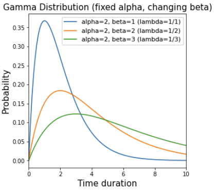
3) Alpha=2, varying beta
This is showing the same horizontal stretch effect (similar to case 1).
For example, the orange curve is really the blue curve stretched by 2x to the right side, and then the height is reduced by 50% to maintain the same AUC.