Approximate Function Methods in Reinforcement learning

Tabular vs Function Methods

In reinforcement learning, there are a few methods that are called tabular methods because they track a table of the (input, output) of the value functions

• Dynamic Programming
  • Policy Iteration
  • Value iteration
  • Generalized policy iteration (GPI)
• Monte Carlo Method
• Temporal Difference
  • Q-learning (Off-policy TD)
  • Sarsa (On-policy TD)

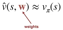
However when the state space is enormous that it cannot be tracked in a table. We can use parameterized functions to approximate these value functions.

• Weight representation is more compact than enumerating all values
• Note that when a weight changes, it can affect multiple outputs (this is similar to supervised-learning)

Linear value function approximation

• The value is approximated using a linear combination of the features
• There are some limitation of expressiveness of linear functions but we can be more creative in making new features
• Tabular value functions are a special case of linear functions
  • Use one weight for each state

Non-linear value function approximation

• Neural network is an example

Generalization and Discrimination

• Generalization: update to value of one state affect value of other states
  • Able to recognize some states are similar to treat them similarly (update both)
  • Extreme generalization: aggregate all state and predict the average
• Discrimination: ability to make value of two states different
  • Tabular methods have high discrimination since it treat each state independently
• Need to find a way to balance the two and make trade-off

Estimate Value Functions as Supervised Learning

• Can we estimate the value functions as a supervised learning problem?
• Supervised-learning
  • Target is fixed. RL has non-stationary target:
    • The environment/policy is not stationary
    • In GPI, we lean the policy and value-function. The target values are nonstationary because of bootstrap.
  • Training examples are batched (not online, temporally correlated)
• Monte-Carlo method can be framed like supervised learning
  • One (state S, return G) mapping for each episode
  • Learn a value function of a given policy
  • Why MC is not supervised learning?
    • Because MC is temporally correlated
• TD can be framed like supervised learning but additional completely than MC
  • Also have (state S, return G) mapping
  • But return G depends on w (target is not fixed)

Value Error Objective

• We want to measure the error between value function approximation and the true value function
• It needs to be weighted different across the state-space using mu(s)
  • mu(s) is often the time spent in state s, known as on-policy distribution
  • stationary in continuing tasks
  • in episodic tasks, mu(s) can depend on the initial state
• mu(s) can be defined as the time spent in each state following the policy pi
• We would like to minimize this value error function by adjusting the weights w
• Can use gradient descent
  • The gradient descent step is followed with Ut replacing v_pi(s) because we are using Ut as an estimate of v_pi because we don’t have true v_pi
  • 
    • If Ut is unbiased, then expected of Ut is v_pi, then we are guaranteed to converge.
  • For linear value function approximation, the gradient is just the feature (each weight corresponds to a feature)
• Even the function that minimizes the error does not mean it’s the true value function
  • Reason is that the function might not correspond to the true value function (limited by the choice of function parameterization and choice of objective/features/functional form)

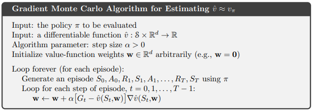
Gradient Monte for Policy Evaluation

• Gradient is quite easy to calculate when the approximation function is linear
• Summing over all states is usually not possible, also hard to know the distribution mu(s)
  • We can make small update each time over the sequence of (state, value) following a policy pi
  • Each step is an update (a form of stochastic gradient descent)
  • Since we don’t have v_pi(s), we can use the sampled return G given state s (G is unbiased estimate of v_pi(s))

• State Aggregation
  • when we update the state-value for one state, the state-value for all the states in the same group is updated
  • it’s a form of linear approximation (the group one-hot variable is the feature)
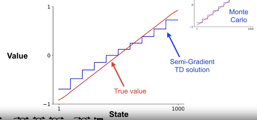
  • Example of a random that takes 100 steps to the left or right of [0, 1000] range. The states are aggregated into 10 states from 1000 states.
  • 

Semi-gradient TD(0) – biased target

• Replace the return estimate with a biased estimate that depends on w (bootstrapping estimate of vi_pi(s))
• It’s not guaranteed to converge because the bootstrapping estimate produces part of a gradient (but something extra depending on w). It’s called semi-gradient methods.
• However,
  • it usually converge quicker because variance is lower
  • it also enables continual and online learning

In the same 1000-state random walk example,

• TD gradient update is biased
• TD runs faster than MC
• Earlier learning is usually more important in practice than long term performance

Linear methods approximation (linear TD)

• Linear in the weights
• x(s) is called a feature vector for state s
• For linear methods, features are basis functions

Update at each time step is

where x_t is just shorthand for x(S_t)

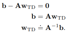
At steady state,

where

The weights must converge to satisfy where w_TD is called TD fixed point.