This is a continuation from Approximate Function Methods in Reinforcement learning
Episodic Sarsa with Function Approximation
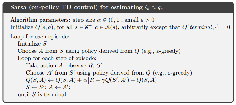
Reminder of what Sarsa is
- State, Action, Reward, State, Action
- On-policy TD Control
- Estimate Q(s, a) by interacting with the environment and updating Q(s, a) each time
To apply it using function approximation in discrete space (stack representation): set up features by crossing the states and actions combinations so that (# of features = # of state-action pairs). This way all combinations of state-action pairs are uniquely mapped, which works for small state-action space.
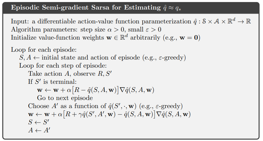
It’s very similar except the Q(s, a) is replaced by the approximate version q_hat(s, a, w)
Exploration under functions approximation
Optimistic Initial Values Causes the agent to explore the action-space because it thinks it will have great return.
- Tabular
- It’s straight forward to implement in the tabular setting but setting an high value in the table for all state-action pairs.
- Function approximation
- Linear/binary – set the weights as high numbers
- Non-linear – unclear how to make the output optimistic. Even if so, it can be influenced by visit to other states that set the weight and affects an unvisited state.
Epsilon-greedy relies on randomness of action to explore the state-action space
- Tabular
- Random spread the probability over the probability epsilon
- Function approximation
- It can be applied but epsilon-greedy is not a direct exploration method.
- Not as systematic as optimistic initial value.
- Still an open area of research
Average Reward
Average reward applies to
- continuing task where the episode never ends
- when there is no discounting (discount rate = 1)
- can be approximated by having large discount rate (0.999) but large sum might be difficult to learn using earlier methods
- reward will be infinite in an episode
- r(pi) = the average reward per time step under policy pi
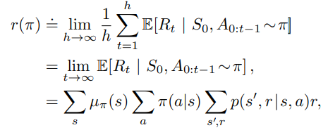
- First expression is the average of time in an infinite horizon
- Second expression is written in terms of expectation
- Third expression sums the reward the probability of state distribution, action given state distribution by the policy, and expected reward over probability transition over state-action pair
Differential Return
Motivating question: this average reward can be used to compare which policy is better. What about for comparing state-action value?
We can use differential return: how much more reward the agent will get from the current state and action for a number of time steps compared to the average reward by following the policy (Cesaro sum)
![]()
To make use of the differential sum, we can let the agent take a different state-action trajectory and then follow the given policy. That will yield some difference in the first few time steps. Showing whether it can be a better policy in terms of positive differential return.
Bellman Equations for Differential Return
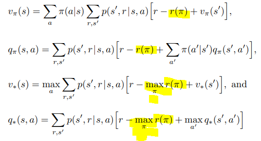
Notice the only difference is that r(pi) is used instead of q() and there is no discounting on the r(pi)
Differential Sarsa

The main differences are
- Need to track an average estimate of the return, but note this is a lower variance update with fixed beta step size
- Differential version of the TD error delta, which is multiplied to the gradient to update the weights w
Preferences-Parameters Confound
Where do rewards come from?
- The agent designer has an objective reward function that specifies preferences over agent behavior (too sparse and delayed)
- The single reward function confounds two roles
- Expresses agent designer’s preferences over behavior
- RL agent’s goal/purposes and becomes parameters of actual agent behavior