What are Chi-squared tests for?
- Compare an expected (hypothesized) categorical distribution vs an observed (sampled) categorical distribution
- Note that the distribution must be categorical (ie. discrete, not continuous)
- Two kinds of common scenarios
- Goodness of fit test
- Test for independence
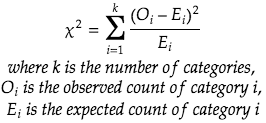
Formula of Chi-square
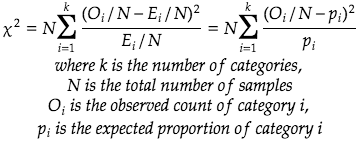
There is also an alternative form expressed in ratio/percentage:
Goodness of fit test
The goodness of fit test tests whether an observed distribution (ie. histogram) comes from a hypothesized distribution at some confidence alpha.
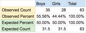
Example 1:
- We want to find out if the population of boys and girl is the same in a school district
- We have a sample of randomly sampled students with 35 boys and 28 girls
- The expected distribution is to have equal number of boys and girls
We can frame the hypothesis test with a significance level of 0.05
- Null Hypothesis: the number of boys equals the number of girls
- Alternative Hypothesis: the number of boy does not equal to the number of girls
Let’s calculate the Chi-squared statistic where k=2 (boys and girls)
![]()
We can look up the Chi-squared value table
- Significant level (p-value) of 0.05 (this is chosen in the set up of the hypothesis test)
- Degrees of freedom = k-1 = 2-1 = 1
Thus the critical value at 0.05 significance level is 3.84. Since the Chi-stat we measure (0.778) is smaller than 3.84, we cannot reject the null hypothesis. This is the same as saying we cannot prove that the boys and girls populations are unequal at the school district.
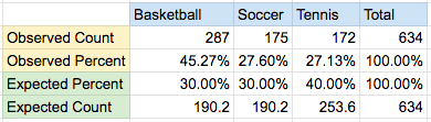
Example 2
This test can apply for more than 2 categories. Let’s say we expect a town to have 30% basketball players, 30% soccer players, and 40% tennis players. We collected random sample as the following:
We test the similar hypothesis as before
- Null hypothesis: the number of basketball, soccer, tennis players follows a 30%, 30%, 40% split
- Alternative hypothesis: the number of basketball, soccer, tennis players does not follow a 30%, 30%, 40% split
We can carry out the same calculation as before
![]()
With 2 degree of freedom (k=3) and 5% significance level, we can look up the critical value again from table which is 5.99. Since 76.74 is larger than 5.99, we can reject the null hypothesis.
Test for independence (or association)
While the goodness of fit tests above are quite simple, the test for independence (sometimes known as test for association) deals with 2 categorical variables. But the idea is very similar, we are still comparing the observed and expected distribution. We also use the same Chi-squared stat formula but across a joint-distribution space.
Example 3
We randomly sample some cars in the city and want to find out if the color of the car is independent from the type of vehicle. Below is the raw data collected
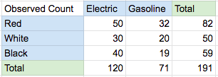
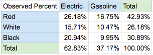
The 2 type cars (electric & gasoline) and 3 colors (red, white & black) give 6 possible combination as shown in the table above. Next we calculate the percentage of the total of 191 cars by divide the entire table by 191.
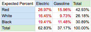
Then we calculate the expected count for the 6 combinations using the subtotals using an independence assumption. This is done by multiplying the marginal probability of the car type by the car color:
Ex: P(Red and Electric) = P(Red) * P(Electric) = 42.93% * 62.83% = 26.97%
We do this for the top 3×2 section
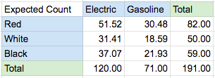
Finally, we convert the entire table from percentage back to count by multiple everything by the total sample size (191).
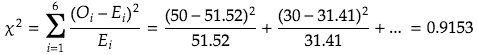
Now we are ready to calculate the Chi-squared statistic using the same formula
The degrees of freedom in this case is product of (number of car types -1) and (number of color -1). So (3-1)*(2-1)=2*1=2. This can be verified by checking the 6 combinations – if we pick the numbers for 2 cells, then all 6 cells are determined

Let Count(Red, Electric)=50, then we can deduce Count(Red, Gasoline)=82-50=32 because we can subtract by the sub-total
Let Count(White, Electric)=30, then we can deduce the following in order
- Count(While, Gasoline)=50-30=20
- Count(Black, Electric)=120-50-30=40
- Count(Black, Gasoline)=59-40=19
Now back to calculate the Chi-squared statistic with 0.05 significance level and 2 degree of freedom from table again.
We see that the critical value is 5.99. Since 0.9153 < 5.99, we cannot reject the null hypothesis that the car type and color are independent from each other.