The normal distribution is one of the most important concepts in statistics and machine learning/data science space. You may encounter the definition through wikipedia or your text book and the memorization of the concepts and formula helps you crack down your exams and interviews, however it might be still unclear what exactly the normal distribution is when you try to refresh your mind on it. In this article, we will introduce the concept with a good example and explain the nuts and bolts for the normal distribution.
Example – Lily’s dates
Lily is sent on blind dates by her friends. She prefer men who is taller than her. She is wondering how many guys are taller than her and what the probability is that. For all her dates, it is likely that there will be few guys who are shorter and few guys are taller than normal, but most of the guys are at around the average height.
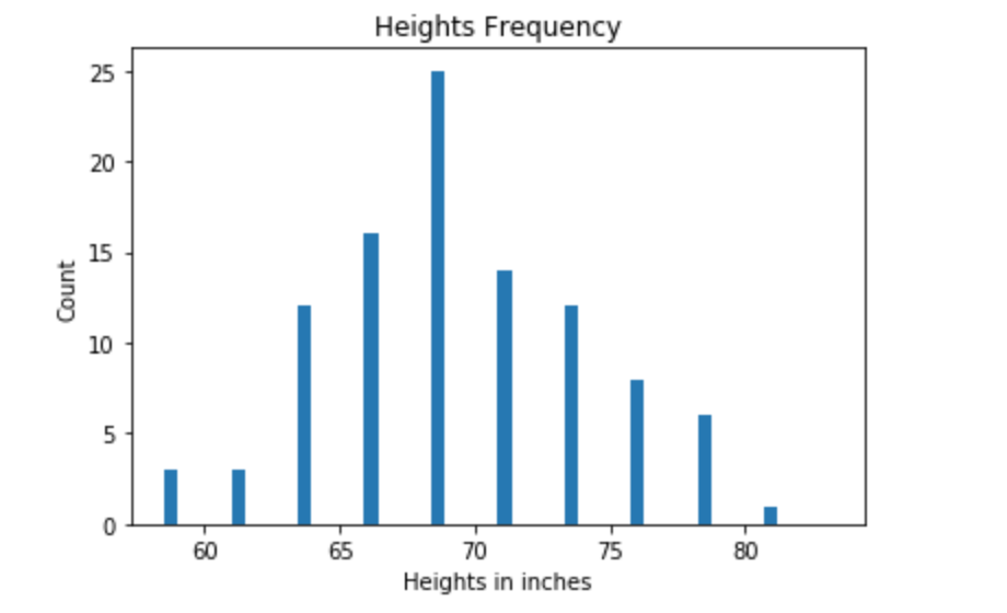
If we plot the heights and frequency, we will get a chart with discrete values like below. X – axis represents the heights. Y-axis represents the frequency (count of guys).
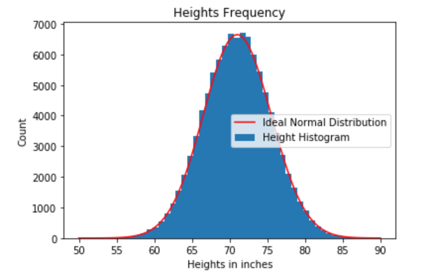
If we extend this to all guys in the town, we will get a bell-curve shape distribution with continuous values like below. It’s called normal distribution.
Definition
Lily’s dates heights can be used as a good example for normal distribution. Here is a more rigid definition you may come across from the text book or wikipedia.
A normal distribution is a continuous probability distribution that is symmetric about the mean, showing that data near the mean are more frequent in occurrence than data far from the mean.
Let’s decompose the definition piece by piece
-
Why it is called “Normal”?
Normal distributions are found widely in the nature and our daily life, especially measurements such as heights, weights, blood pressure, student test scores etc. The normal distribution is called normal as it is seen an ideal pattern of the data and we “normally” expect to see in real life.
2. What is “Continuous”
Continuous refers to continuous data instead of discrete data applied in normal distribution. Chart 1 – heights and frequency shows discrete values distribution, which the values in x-axis are countable. Chart 2 – normal distribution of the heights show that the variables are continuous and infinite on the x-axis and thus those variables compose a line in curve shape. The y axis in the normal distribution represents “possibility density” or “tendency”. The possibility for a precise value in the normal distribution is 0. It may sounds counter-intuitive in the first glance. The precise value requires an infinite number of decimal. Measuring the height to the nearest atom is impossible, therefore it is meaningless to get the possibility for a single precise value in this case, what we really care is to find out probability for a range of values by calculating the area underneath the curve. In other words, only area matters!
3. Probability distribution
A probability distribution is a statistical function that describes all the possible values and probabilities for a random variable within a given range. This statistical function is also called “probability density function”. The function is represented by a formula starting with “f(x)=…” It uses area beneath the curve to tell you about possibilities. We can calculate the area under the curve (cumulative probability) by figuring out numerical calculus integration problem using this function. However, it is very complex of doing this by hand so we look up the area (probability) from the standard normal table by Z-value.
4. Shape and Property
The normal distribution is also known as the bell curve. It is symmetrical and unimodal, with greatest probability density in the center of the curve or (in other words around the mean). The possibility decreases further away from the mean. The curve spreads away from center and approaches to possibility of “0” but never reaches it. You can think of it the way that the events become more and more unlikely but there’s always a tiny chance they might. The total area under the curve equal to 1, or in the other words, the total possibility that equals the sum of the likelihood of each individual event is 1. Please remember this, it is an very important property that we will use to solve series of possibility related problems later.
5. Decipher the Formula
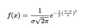
The normal distribution function is defined by the formula below. The formula is a mathematical representation of the bell – curve. Do not be bothered by the complexity of it. Since both e and pai are constants, the function is completely defined by only 2 parameters, mu and sigma.
Mu is also known as population mean, which defines the position or the center of the curve. Sigma is also known as standard deviation, which defines the wideness or how spread the curve is.
You do not need to memorize the formula but keep in mind you need Mu and sigma to define the curve (which is the key for most problems).
Standard Normal Distribution
Standard Normal Distribution is a special normal distribution where the mean is 0 and the standard deviation is 1 (mu = 0, sigma =1).
Why standard normal distribution is important? It’s important for convenience. In order to calculate the probability that a normal distribution random variable smaller than a given value, you can transform the random variable to a standard normal because typically only the table for standard normal is provided. (There are infinite of pairs of mu and sigma, thus there will be infinite tables!)
For most of the probability problems, we need to transform the variable X (if it follows normal distribution) to a standard Normal Distribution, so we can look up the table to calculate the probability that X is smaller than a given value.
Find normal possibilities
Jumping back to the example of Lily’ dates in the beginning. We can help Lily to find out how many guys are taller than her and what the probability is that. Let’s summarize from the notes earlier and known factors here.
- Total area underneath normal distribution curve is 1
- Lily is 64 inch. (This is given)
- The mean and standard deviation of the height for the guys in town are 71 inch and 4.5 inches (variance equal to 22.5, which is calculated as the square of the standard deviation). (This is given). We use notation X~(mu=71, var=20.25) to represent the distribution and it is read as “random variable X follows a mean of 71 and a variance of 20.25”
- Now we need to transform the X to a standard normal distribution Z.
- Look up the standard normal table
first, we move the mean from 71 to 0 so we subtract 71 from X to get to 0, then we squeeze the width from 4.5 to 1 thus we divide 4.5. Doing this gives you (X-71)/4.5 we call this value as Z score or standard score because (X-71)/4.5 now follows mean of 0 and variance of 1. In our case, we want to find the probability Lily’s dates are taller than 64, we need to find out P(X>64), so we want to know the area beneath the curve on the right side of 64.
So we rewrite P(X>64) as P((X-71)/4.5) > (64-71)/4.5) by applying the transformations above. This is now P(Z > (64-71)/4.5) since (X-71)/4.5 is the same as standard normal distribution Z. Evaluation the right side, we have P(Z>-1.56). Next we rewrite it again using the “right tail” probability as P(Z>-1.56) = 1 – P(Z<-1.56).
Look up the probability from z score table so we have P(Z<-1.56) = 0.05938, so P(Z>-1.56) = 1-0.05938=0.9406