
If you are preparing for data science interviews, you will likely encounter one of these models.
-
- Nearest Centroid
- K-Nearest Neighbors
- Naive Bayes
- Decision Tree, Random Forest, and Boosted Tree
- Support Vector Machine
- Neural Network
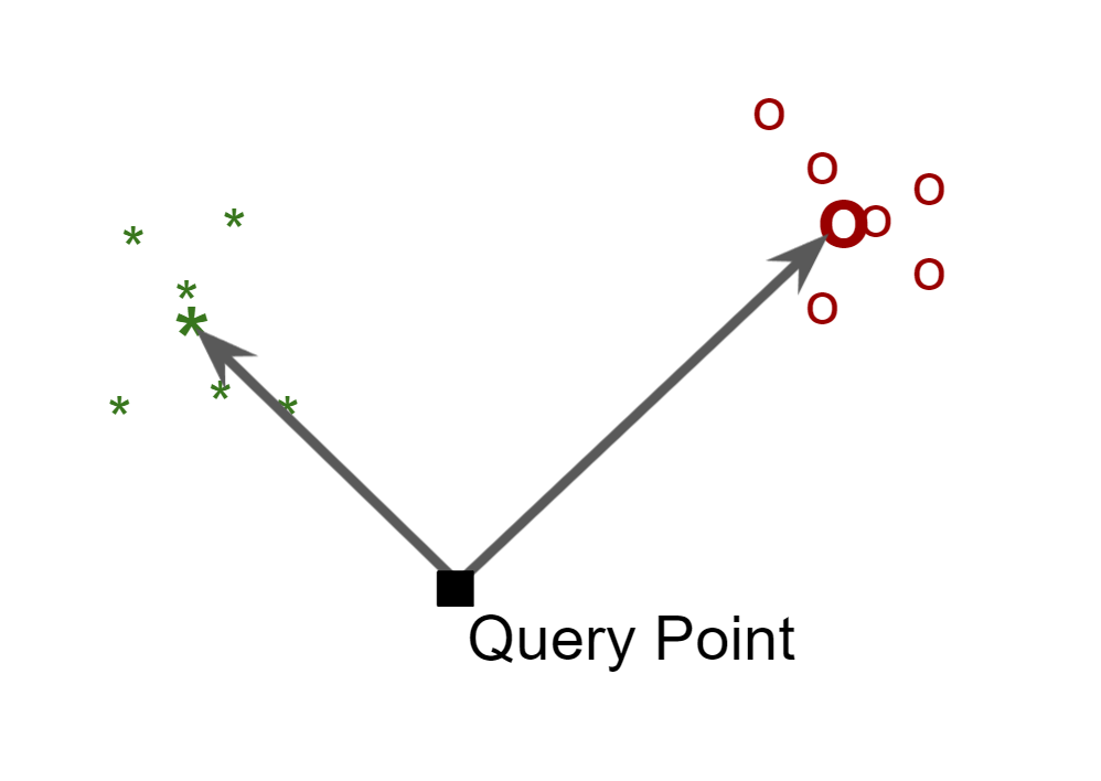
Nearest Centroid
The nearest centroid is one of the most simple model, and it works as the follow
- Compute the mean (centroid) of all the sample for each label
- Predict the class by the identifying the centroid that is closest of the query point in the feature space
Pro:
- Most intuitive model
- Fast to train and evaluate
Con:
- Only works for very simple data where data is easily distinguishable
Chances of encountering in data science interviews: ★★
- Not because it’s too simple, but because people often have forgotten about it.
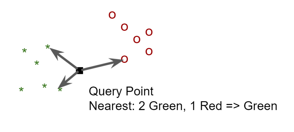
K-Nearest Neighbors
The K-nearest neighbor requires no training. It just predict the classification of the query by gathering the k nearing point in the feature space, and decide the classification by voting among these points.
Pro:
- Simple to understand
- Takes zero time to train
Con:
- Can be slow during prediction when the number of training example is large
- Performance tends to weaken as the number of feature increases
Chance of encountering in data science interviews: ★★★
- It can often be brought up as the very first solution when working out a test case.
Naive Bayes
The Naive Bayes classifier involves some probability theory from the Bayes Theorem.
We first start by stating that each feature might have some correlation with the label that we are trying to predict. This correlation is bi-directional, which means
- Observing the feature can inform you something about the probability distribution of the label
- Vice versa, observing the label can also inform you something about the probability of the feature
The Naive Bayes classifier makes a naive assumption that each feature influences the label independently and thus we can multiply conditional probability of the label on each feature to get the conditional probability of the label on all feature jointly.
Ex:
We would like to classified a person as male (class 0) or female (class 1) based on the 2 features
- Feature 1: whether the person wears a dress
- Feature 2: whether the person wears a hat
| Label (y) | Feature 1 (wears a dress) | Feature 2 (wears a hat) |
| 0 | False | False |
| 1 | True | True |
| 0 | False | True |
| … | … | … |
| 1 | True | True |
| 1 | False | False |
Without making any assumption, if we are given a person who wears a dress and also wears a hat, we can make prediction about the label of the person by comparing
- A1) P(y=0 | Feature 1 is True AND Feature 2 is True)
- A2) P(y=1 | Feature 1 is True AND Feature 2 is True)
If (A1) > (A2), we classify the person as male (y=0), else as female (y=1)
Instead of doing the above comparison, we first apply Bayes Theorem to express the probability in an invert form:
- B1) P(Feature 1 is True AND Feature 2 is True | y=0) * P(y=0) / P(Feature 1 is True AND Feature 2 is True)
- B2) P(Feature 1 is True AND Feature 2 is True | y=1) * P(y=1) / P(Feature 1 is True AND Feature 2 is True)
Notice the denominator of (B1) and (B2) are the same, so we can remove it without affecting the comparison
- C1) P(Feature 1 is True AND Feature 2 is True | y=0) * P(y=0)
- C2) P(Feature 1 is True AND Feature 2 is True | y=1) * P(y=1)
Next step is the key part, we apply an independence assumption between Feature 1 and Feature 2 (this is what is Naive about the Naive Bayes method).
- D1) P(Feature 1 is True | y=0) * P(Feature 2 is True | y=0) * P(y=0)
- D2) P(Feature 1 is True | y=1) * P(Feature 2 is True | y=1) * P(y=1)
At this point, you might be wondering about a few things:
- Q: Why is this assumption valid? How do we know if it’s true?
- A: Actually we don’t know, but we are hoping so. But depending on how much Feature 1 and Feature 2 are correlated, it will impact the performance of the model
- Q: Can’t we just calculate (A1) and (A2) directly anyway? Why do we prefer (D1) and (D2)?
- A: The reason is (D1) and (D2) are easier to compute. (A1) and (A2) are joint probability. Image if we have 20 binary features, we would need to estimate pow(2, 20) = 1 million probabilities (think about all possible combinate of Feature 1 to 20). On the other hand, for 20 features, there are only 20*2 = 40 probabilities to estimate (only need to estimate P(Feature1|y=0) and P(Feature 1|y=1) for Feature 1 to 20).
As a result, the Naive Bayes method is very efficient computationally and in the right circumstance, it can provide great predictive problem (such as traditional email spam filtering)
Pro:
- Efficient to compute
- Still effective in many practical situations
Con:
- Independence assumption is too strong leading to bad performance in many circumstance
Chances of encountering in data science interviews: ★★★★
- It’s actually quite a popular question to ask because of it wide use in practice.
- It also allow the interviewer to test your probability skills.
Decision Trees, Random Forests, and Boosted Trees
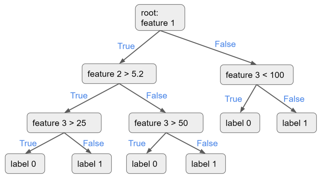
Decision Tree
Decision is represented as a set of node where you can traverse from the root node until you read a leaf node.
Training: A decision tree is trained iteratively to result in the topology above with each node representing a decision.
Prediction: You traverse the tree from the root node on the top by evaluating at each decision.
Pro:
- Easy to understand and explain
- Fast to execute and evaluation
- Generally robust to outliers
Con:
- Prone to overfitting
- Can get messy if there are many dimension
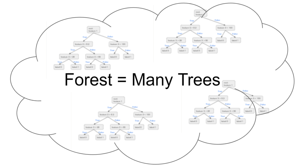
Random Forest
The Random Forest model takes the Decision Tree model to the next level by bagging many trees into a forest. Each tree is trained similar to the training of a Decision Tree but with randomness injected to the training process to make sure the trees are not too similar. The prediction process is basically an averaging of the result from all the trees.
Pro:
- Much more robust and Decision Tree
- Reasonably high accuracy and usually used the first model when a data scientist faces a new problem
Con:
- Training and prediction can be slowed down as we increase the number of trees
- There can be still some correlation among the trees
- It is harder to explain and understand with a large number of trees
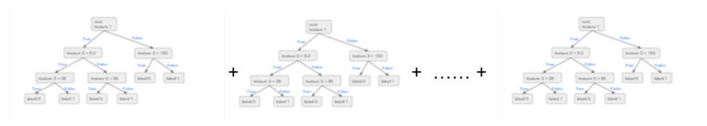
Boosted Tree
The Boosted Tree model is similar to the Random Forest model because it also use many Decision Trees. However, instead of training them as independent trees, it trains each trees in sequence which each tree enhances (boosts) the misprediction from all the trees before it. There is also mechanism to reweight the sample differently in each iteration so that the subsequent tree can “focus” on the samples that cause misprediction.
Pro:
- Prediction accuracy is the highest among all classical model
- Relatively quick to evaluation
- Still relevant today in many applications
Con:
- Training can be slow compared to Random Forest because it trains each tree sequentially
Chances of encountering in interview: ★★★★
- Tree models are so widely used.
- Although tree models are no longer the state of the art, they are quite popular in practice.
Support Vector Machine
The SVM model is the go to model before deep learning. The training process is to find a margin maximizing hyperplane to separate the 2 classes. In short, the SVM model can be summarized as


It’s an be solved by formulating as a quadratic programming problem. It also have a few extension such as kernels and soft margin. The detail is beyond the scope of this post, so I would just skip it for the time being.
Pro:
- Good prediction performance
- Fast evaluation speed
Con:
- Works well for binary classification but has to tweak a bit to work for multi-classification
Chance of encountering in data science interviews: ★★★
- It lost some popularity because of the rise of deep learning model.
- It is not quite suitable for large amount of data but it’s still used as a last stage that can process the result from a deep learning model.
Neural Network
Neural Network is also knowns as Artificial Neural Network. It’s inspired by the biological neuron of the brains. It has a graphic representation where each node can take in multiple weighted input (fan-in) and transmit the result to other nodes (fan-out). It’s typically organized as Input/Hidden/Output layers as below:
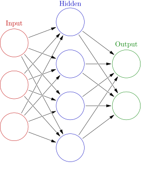
- The number of nodes in the input layer represent the number of features.
- A deep network means there are multiple hidden layers.
- The output layer should be just 1 node for a binary classification problem.
Note that each arrow in the diagram actually represents a weight from the node in the previous layer to the next layer. Within each node, there is typically an non-linear activation function. In a classification problem, it typically uses a sigmoid node at the last layer, and the objective function is usually the cross entropy as defined below:

The common training process of a neural network is thru gradient descent with a trick called back-propagation. There are quite a few details that is involved in solving this optimization problem of finding the optimal weights in the arrows to achieve the minimal prediction error over all training example.
- The cost function – this is the cross entropy loss function above
- The learning rate – how big of a step size to take each iteration
- The optimizer (ex: Stochastic Gradient Descent, Adam, Adadelta) – this control the adaptiveness/momentum of the learning
- The batch size – how many training samples to use in each iterations
- Epoch – how time times we want to iterate the entire training data set
- The structure of the network – how many layers, how many nodes per layers.
- Weight Initialization – bad initialization can cause a network to fail to converge. This was actually a main reason why Neural Network “did not” work for a long time in the past.
- Choice regularization – L1, L2, drop-out layers, data augmentation.
Further, there are many variants of NN such as Convolutional Neural Network and Recurrent Neural Network. They can have much better performance compared to vanilla Feed-forward Neural Network described above.
The evaluation of Neural Network also tends to be more extensive because we still don’t have a good understanding and have to treat it like a black box often. This means we need to apply a lot more caution when validating the model.
There are just too many things to talk about NN but I would stop here in this post.
Pro:
- Achieve state of the art accuracy
- Able to improve from large amount of data
Con:
- Hard to interpret/explain
- Resource intensive both in computing and data volume
Chances of encountering in data science interviews: ★★★??
- If you are applying to Machine learning position, then you will probably encounter Neural Network.
- If you are just applying for data analyst position, you might not encounter it at all.