Model Interpretability

Defintion

Explainable Artificial Intelligence (XAI) is a field of AI to provide transparency and details on the decision making process of the AI system.

Interpretability – the amount of effort for a human to understand the model

Why

• Ensure fairness in the algorithm
• Identify bias in training data
• Model monotonicity can help with interpretability
  • Ex: Tensorflow Lattice Model (TFL)
• Debugging/testing the model
• Especially more important for sensitive model such as NLP where it can generate wildly incorrect results
• Monitor vulnerability to attacks
• Affect the reputation and branding of the product when you can explain to customers and stakeholders
• Legal and regulatory – when model is challenged in court for example
• Answer questions about bad results from adversarial attack
  • Identify the perturbation that fooled the model

Interpretability Methods

• Intrinsic vs post-hoc
  • Intrinsically interpretable: linear, tree-based, lattice models
  • Post-hoc: applied after training, treat model as blackbox
    • Feature importance
    • Partial dependence plot – relationship between target and a set of features while marginalizing all other features
      • 
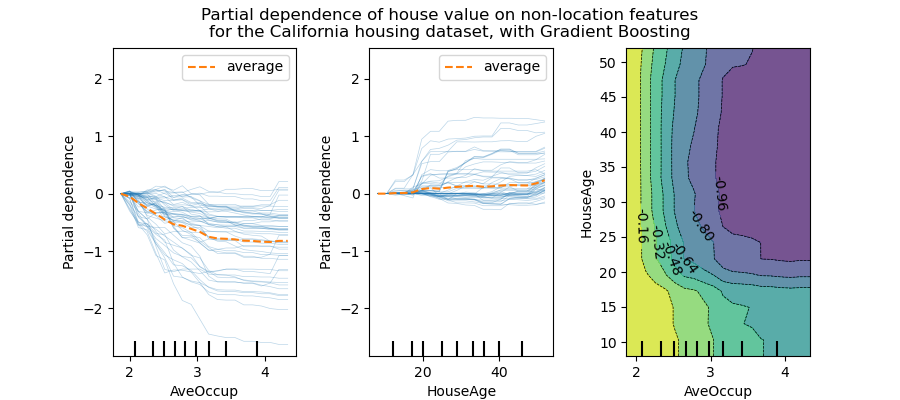
      • Advantage: easy to interpret and visualize
      • Issues of PDP:
        • Human can only visual it up to 2 dimensions
        • create impossible sample
        • Assume features are not correlated: only isolated effects (does not work right with correlated features)
    • Permutation Feature Importance
      • Measure the increase in prediction errors after permuting the feature
      • A feature is important is shuffling its value increases model error
      • Perform on each feature individually and order the feature by the model error
      • Advantage:
        • Easy to interpret
        • Global insight of the model
        • Does not require retraining the model
      • Disadvantage:
        • Unclear whether to use training data or testing data to measure it
        • Does not work well with correlated features (similar to PDP)
        • Need access to label data
• Model specific vs model agnostic
• Local vs global
  • Local – explain an individual prediction
    • Feature attribution
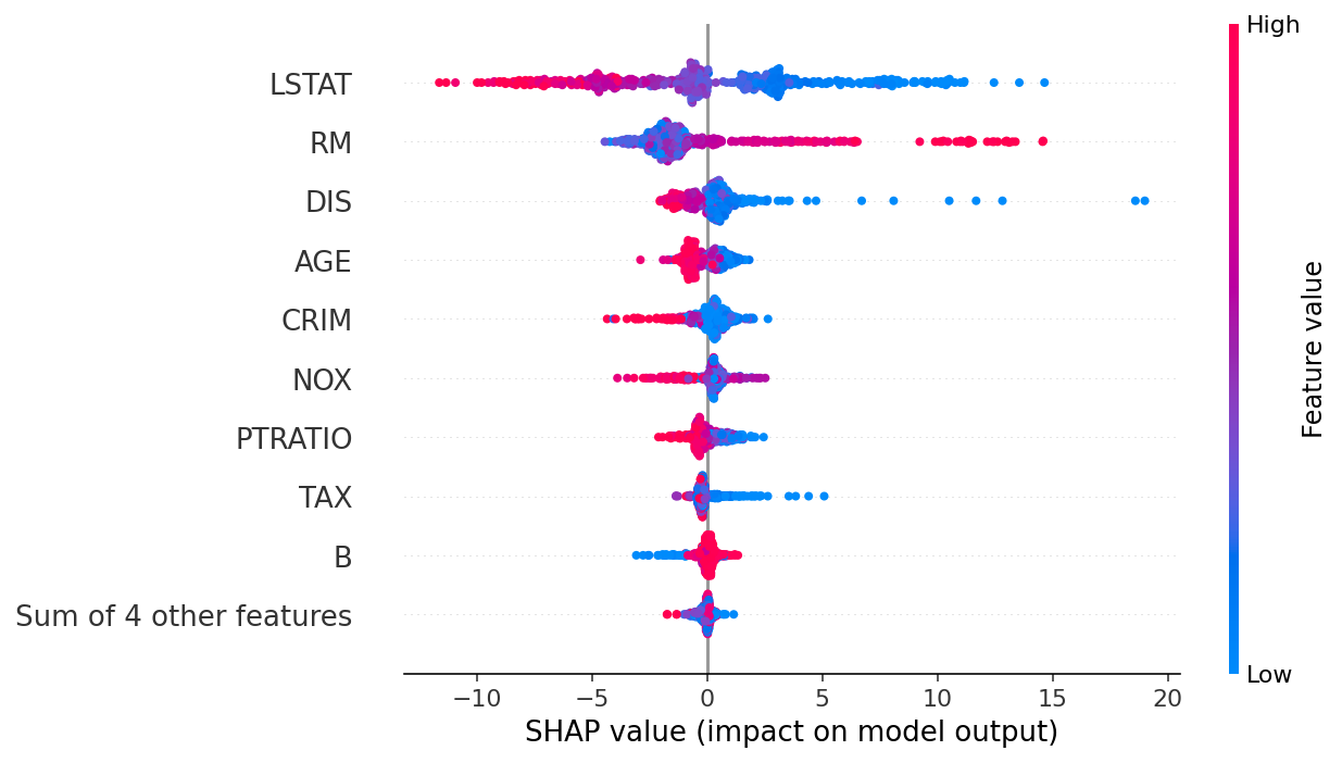
      • Shapley Values
        • 
        • Definition of Shapley Value: in game theory, a group of player in a cooperative game, how do you assign payout to the each player according to his/her contribution?
          • In ML, Players = Features, Pay = Prediction Diff from Mean
        • Has solid theoretical foundation
          • Might be the only legally compliant method to distribute the contribution fairly
          • Able to contrast to sub-population
        • Disadvantages of Shapley Values
          • Computationally expensive
          • Cannot selectively only interpret some features (must run for all features)
          • Cannot do what-if by change an input feature
          • Does not work well when features are correlated
        • Steps
          • Step 1: Get random permutation of the features (reorder the feature columns)
          • Step 2: Get a random sample from dataset
          • Step 3: Generate 2 samples from the chosen one above
            • Sample 1: resample the value after the interested feature
            • Sample 2: resample the value at and after the interested feature
            • Intuitions
              • What is the difference going from any other values to the one we are interested in?
              • Similar to PDP but since the values after the interested feature is also changing, it’s less artificial than PDP
          • Step 4: repeat steps 1 to 3 and average the difference
            • Intuition: the difference is the contribution of the interested feature at its current value from the base value (which is the just the mean target value of the training data)
      • SHAP vs Shapley values
        • SHapley Addictive exPlanation
          • TreeExplainer
          • DeepExplainer
          • GradientExplainer
          • KernelExplainer
        • Combines with LIME for local explainability
      • LIME – Local Interpretable Model-Agnostic Explanation
        • Local – Explain one instance at a time
        • Generate random perturbations around the instance n times
        • Requires Retraining – Fit a linear (or just any simple) model on these n points (local surrogate model)
        • Use distance from the instance to signal importance and convert it to weight using kernel function (exponential)
        • The result is a linear boundary mostly influenced by the near by points and the coefficient of the linear model can explain the impact of near the local instance
      • Saliency Map
        • Measures the importance of each pixel to the prediction
        • Use the first-order derivative of the probability of a class w.r.t. a pixel value
      • TCAV – Testing with Concept Activation Vectors
        • The goal is to determine how much a concept (e.g., gender, race) was necessary for a prediction in a trained model even if the concept was not part of the training.
        • Key
          • the concept is high-level (human level) not low-level (pixel level)
          • speak to the users at their language so that users don’t have to learn ML to interpret the model results
        • TCAV can provide an explanation if TCAV is trained on this concept
          • Training TCAV: to learn CAVs (Concept Activation Vectors)
          • Input: examples of concept (ie. images with stripes to learn the stripe concept)
          • Need access to the internal activations of the network
          • Train a linear classifier to separate the activations of random images from the concept images
            • The activations can be taken from any layer of the network network
          • The vector that is orthogonal to the decision boundary is the CAV
            • Similar to word2vec where gender vector = man – woman
          • To get a TCAV score from an image w.r.t a concept
            • Take the derivate of the prediction output of a class (ie. zebra-ness) along the CAV
            • If we make this image more like the concept (ie. stripes), how much more does the classifier predict that particular class (ie. zebra)
          • Final score, run this over all zebra images, check percentage of zebra images that responds positive to the concept vector overall
        • How do we know if the CAV is sensitive and we are getting results by chance?
          • Repeat the random image selection and calculate new CAV
          • Calculate the score for each CAV
          • Get a distribution of the CAV scores
          • Compare this against CAV score of full random images against random images
          • Get another distribution of the CAV scores
          • Check the two distributions above are statistically significantly different (t-test)
  • Global – feature contribution over the entire dataset
    • Perform Shapely value calculation above over all samples in the dataset and average the result
    • 

Tools

Google AI Explanation

• Return both prediction and explanation from AI Platform
• Feature attribution methods used by AI Explanation
  • Sampled Shapley
    • For non-differentiable model
    • Very flexible but less efficient to compute
  • Integrated Gradient
    • More efficient to calculate than Shapley
    • Integrated is method to calculate the gradient of the sample along an integral path
      • Early interpretability methods for neural networks assigned feature importance scores using gradients, which tell you which pixels have the steepest local relative to your model’s prediction at a given point along your model’s prediction function.
      • However, gradients only describe local changes in your model’s prediction function with respect to pixel values and do not fully describe your entire model prediction function.
      • As your model fully “learns” the relationship between the range of an individual pixel and the correct ImageNet class, the gradient for this pixel will saturate, meaning become increasingly small and even go to zero
      • The intuition behind IG is to accumulate pixel x’s local gradients and attribute its importance as a score for how much it adds or subtracts to your model’s overall output class probability
        • Interpolate small steps along a straight line in the feature space between 0 (a baseline or starting point) and 1 (input pixel’s value)
        • Compute gradients at each step between your model’s predictions with respect to each step
        • Approximate the integral between your baseline and input by accumulating (cumulative average) these local gradients.
  • XRAI – eXplanation with Ranked Area Integrals
    • Combines the integrated gradients method with additional steps to determine which regions of the image contribute the most to a given class prediction
      • Calculate pixel-level Integrated Gradients
      • Oversegmentation of image to create patches of the image
      • Aggregate pixe-level IG at each segment to determine density, rank each segment to determine more salient/contributing area