Lagrange Multiplier Explained

Goal

Gradient descent seems to work fine for finding the local maxima and minima of a function, and Lagrange Multiplier helps to find the local maxima and minima with constraints.

You can read about the definition in Wikipedia, but I am going to focus on explaining the intuition in the rest of the article. Going from simple to complex examples to demonstrate the benefit of using Lagrange Multiplier.

Unconstrained optimization

• This problem can be solved by checking the first order conditions
  • 
  • Take the partial derivatives with respect to x and y
  • Setting those partial derivatives equal to 0.
  • Solve this system of equations with 2 equations and 2 unknown.
  • Note that it’s not always possible to get a closed form solution.
• You still need to check the second order condition – determinant of Hessian should be greater than 0
• It’s possible that that the function is unbounded, then there would not be a maximum

Problem with equality constraint(s)

• In some problem it’s possible to rearrange g(x, y) to express x in terms of y or y in terms of x.
  • Then substitute the above expression back to f(x, y) to solve as an unconstrained optimization problem.
  • This can work in some limited case but would be very difficult when g(x, y) is a more complicated function.
    • Ex: hard to solve for x or y on one side the equation:

Time to try out the Lagrange Multiplier, by definition

The first order condition is

Let’s try to apply Lagrange Multiplier in a simple example that can be solved analytically:

First recognize the f(x,y) and g(x,y) of this problem by matching with the standard form, we can write out L as

Next take the partial derivative to get the first order conditions

Intuition: another way to interpret this first order condition is that we are trying to match the gradient of f(x,y) with lambda multiplied by the gradients of g(x,y). Since lambda is a scalar, these two gradient vectors must be point at the same directly or in complete opposite direction (if lambda is negative). This is true iff the contours of f(x,y) and g(x,y) are tangential.

FOC in vector form,

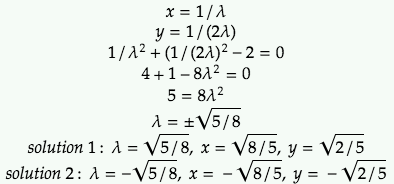
Solving the stationary points with the 2 first order condition equations and the original g(x, y)=0

Check the second order condition (Hessian Matrix) for solution 1:

Calculate the determinant

Since det(H)>0, H is positive semi-definite. This is true for all values of x,y over the entire R2 plane. So solution 1 must be local maximum/minimum. When the top level element of H is negative, this means solution 1 is local maximum.

Perform the same calculation for H with solution 2, we can similarly find that det(H) = 5/2 also, but the top left element is positive, which means solution 2 is a local minimum.

Since there are the only 2 critical values, solution 1 is the global maximum.

Intuition: lambda is positive in both solution which means g(x,y)=0 is a binding constraint as expected. We can explore the case of inequality constraint in the next example below.