Understanding eigenvalues, eigenvectors, and determinants

What are eigenvalues and eigenvectors?

We have to answer both concept together since they are closely related?

• Given a square matrix A
• If we find a vector v such that A*v = lambda * v
  • where lambda is a scalar value (not a vector)
  • then we call v an eigenvector of the matrix A and lambda the associated eigenvalue
• Intuitively, find a vector that can be multiplied to the matrix as if just apply simple scalar multiplication, which is really just stretching the vector to be long/shorter (or flipping).

Determinant

The signed area of the parallelogram stretched by the eigenvectors of matrix A equals to the determinant.

• Note that this area can be negative when a eigenvector is negative
• Note the area is 0 when the matrix A is rank deficient (it does not stretch into a full volume in the n-dimensional space)
• In the context of a Hessian matrix H, the determinant of H tells whether the function is convex
  • When the det(H) > 0, the signed area is positive, which sort of represents a bowl shape
    • Upward bowl is convex when the diagonal is positive
    • Downward bowl is concave when the diagonal is negative
  • When the det(H) < 0, the signed area is negative, which represents a saddle point

Why do we care?

This is very important in understand many optimization method in solving ML problems today

• Gradient Descent
• Secant Method
  • BFGS (Broyden–Fletcher–Goldfarb–Shanno algorithm)
• Principal Component Analysis
• Singular Value Decomposition

What is Principal Component Analysis (PCA)?

PCA is a way to decompose a square matrix A by finding eigenvalues and eigenvectors.

• It does so by finding eigenvectors that are orthogonal to each other.

• If X is our data where each row is a sample, and each column is a feature. Assuming X is demeaned, then Q is the covariance matrix.
• We decompose the matrix Q in 3 parts: W, lambda, transpose(W)
• Each column of W is an eigenvector.
• Lambda is a diagonal matrix where the elements along the diagonal are the eigenvalues

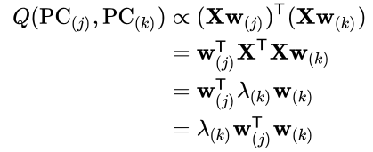
• One interpretation is to ask what is the covariance between the j-th principal component and the k-th principal component.
• w(j) is the eigenvector at j-th component
• w(k) is the eigenvector at k-th component
• This result should be zero for PCA because we ensure the eigenvectors are orthogonal

If we look at this formula again, it says that W (the eigenvectors) are scaled by the lambda (the associated eigenvalues), and then multiplied by W-transpose (the eigenvector) again. Since each eigenvector (component) is orthogonal, the result is basically the same of these rank-1 spaces represented by each component.

• The larger eigenvalues represent more variance of the data in the direction of the associated eigenvector.
• If we only keep the large eigenvalues by removing the small eigenvalues and their eigenvectors, then we can still represent the original matrix Q with good approximation.

Interpretation

• Q is seen as a system that takes a vector of n-dimension to another vector of n-dimension
• W is a projection of the input vector into the eigenspace
• Lambda is scaling applied to each dimension in the eigenspace
• Transpose(W) is a project of the vector in eigenspace back to the original input space

What is SVD?

The Singular Value Decomposition algorithm is another method to decompose a matrix very similar to the PCA.

X is an m by n matrix

U is a complex unitary matrix (m by m)

• The (conjugate) transpose of U is also the inverse of itself, so U*transpose(U) = I.
• U is a square matrix
• Columns of U forms an orthonormal basis of the space of dimension m
• All the eigenvectors of U are orthonormal to each other and lie on the unit circle

Sigma is a diagonal matrix (m by n)

• The values along the diagonal are called the singular values
• non-negative
• The

W is a complex unitary matrix (n by n)

• The (conjugate) transpose of W is also the inverse of itself, so W*transpose(W) = I.
• W is a square matrix
• Columns of W forms an orthonormal basis of the space of dimension n
• All the eigenvectors of W are orthonormal to each other and lie on the unit circle

Interpretation

• X can be seen as a system to take n-dimensional vector as input to a m-dimensional vector as output.
• U and W represent the basis of the input and output spaces respectively.
• Since U and W are orthonormal, they don’t apply any scaling. The diagonal matrix (sigma) provides the scaling functionality of this system.
• Each of these operations is analogous to the PCA case except SVD is more applicable to even rectangular matrix (different input and output dimension)

How is SVD related to PCA?

When the matrix is positive semi-definition square matrix (ie. a covariance matrix), PCA and SVD yield the same decomposition.