A Practical Data Science Case Study: Free Housing Data

What is free housing data?

Let’s say you are interested about investing in the real estate market and want to learn about the trends. You can:

• Ask your friends where to buy a house
• Ask your local real estate agent
• Ask google
• Read the news paper

Sure, all these option will provide you with some information. But do you want to know how to find out yourself?

This is exactly the goal of this article: to show you the “data scientist” way to find out yourself!

Why should you read this article?

• To learn about how to utilize open/free housing data
• To learn about how to practice data science in the real world
• To get inspirations to start on other data science project you like
• To demystify the process of turning raw data into analysis

First, download the free housing data!

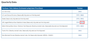
There are many open (free) dataset out there about the US housing market. We are going to use the open data provided by the Federal Housing Finance Agency (www.fhfa.gov).

They list plenty of data sets on their website: FHFA website

These data are published periodically and you have a lot to explore.

We can first down the data set “100 Largest Metropolitan Statistical Areas (Seasonally Adjusted and Not Adjusted)”

Pre-requisites:

• Python: beginner level
• Jupyter Notebook: know how to launch it

If you are not familiar with the pre-requisite, you can skip the code snippet and just focus on the chart produced by the code!

My goal is to encourage you to explore to learn about Python and data science in the future!

Plotting 30 year trend of the top 100 metro

The below code snippet does a few thing to plot the data:

• load data from Excel
• preprocess the time axis with (year + quarter)
• plot the each metro as its own curve in the plot

import pandas as pd
import matplotlib.pyplot as plt
from matplotlib.pyplot import figure

# load the data
df = pd.read_excel('HPI_PO_metro.xls')

# preprocess the time axis by combining the year and quarter
df['Q'] = df.yr.astype(str) + "-Q" + df.qtr.astype(str)

# plot the data
fig, ax = plt.subplots(figsize=(15,12))
for metro, g in df.groupby(['metro_name']):
    ax = g.plot(ax=ax, kind='line', x='Q', y='index_sa', alpha=0.5)
    ax.get_legend().remove()

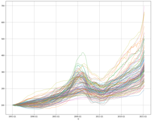
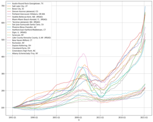
Observations from the chart:

• The data runs from 1991-Q1 to 2021-Q2 (about 30 years)
• The value on the y-axis is the housing price index where all metros start at 100 in 1991-Q1
• There is a large jump around 2006, followed aby a large drop in 2008.
• Most metros reach the bottom around 2011 and have been in a strong growth trend after 2011 to 2021-Q1
• While all metro starts at 100 in 1991-Q1, the growth trajectories are quite diverse. The top metro has gone to 700 while the bottom metro has bar

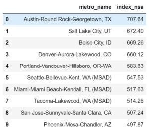
Getting the top 10 and bottom 10 metros:

It’s still quite hard to tease out the chart because we have 100 curves overlay on top of each other. We can focus on the top 10 and bottom 10 metros next.

• Sort the metros by their prices in 2021-Q1
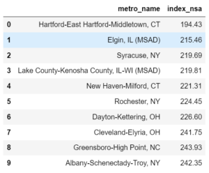
• Retrieve the top 10 and bottom 10

# Top 10 Metro
df_top10 = df[df.Q == '2021-Q2'].sort_values(['index_sa'], ascending=False).head(10)
df_top10[['metro_name', 'index_nsa']].reset_index(drop=True)

# Bottom 10 Metro
df_bottom10 = df[df.Q == '2021-Q2'].sort_values(['index_sa'], ascending=True).head(10)
df_bottom10[['metro_name', 'index_nsa']].reset_index(drop=True)

• Replot these 20 metros with legend

# set image size
fig, ax = plt.subplots(figsize=(15,12))

# iterate top 10 metros
for metro in df_top10.metro_name.values:
    ax = df[df.metro_name == metro].plot(ax=ax, kind='line', x='Q', style='-', y='index_sa', alpha=0.8, label=metro)

# iterate bottom 10 metros
for metro in df_bottom10.metro_name.values:
    ax = df[df.metro_name == metro].plot(ax=ax, kind='line', x='Q', style='--', y='index_sa', alpha=0.8, label=metro)

# style the grid
ax.grid('on', which='major', axis='x' )
ax.grid('on', which='major', axis='y' )

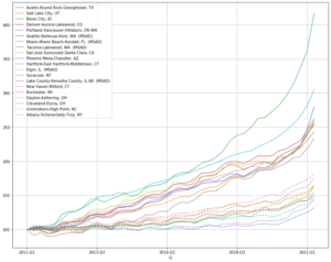
Now it’s much more clear to compare the 2 categories of metros

• By looking at the legend on the upper left corner, we recognize many of the familiar names of the hottest metros
• It seems like the top 10 metros over the 30 years also have the biggest dip in the 2011, but they all bounce back. In contrast, the bottom 10 metros experienced some similar dip but did not quite bounced back.

Zoom into 10 Year Trend

To validate the 2nd point mentioned about the bounce back post 2011, we can further explore the data by renormalizing the index at 2011.

# set up the base value at 2011-Q1
base_values = df[df.Q == '2011-Q1'].set_index('metro_name')
base_values_dict = base_values['index_nsa'].to_dict()

# normalize the index by the 2011-Q1 value
def normalized_2011(row):
    metro = row['metro_name']
    base_value = base_values_dict[metro]
    return row['index_nsa'] / base_value * 100
df['index_nsa_normalized'] = df.apply(normalized_2011, axis=1)

# plot the result
fig, ax = plt.subplots(figsize=(15,12))
for metro in df_top10.metro_name.values:
    ax = df[df.metro_name == metro].plot(ax=ax, kind='line', x='Q', style='-', y='index_nsa_normalized', alpha=0.8, label=metro)
for metro in df_bottom10.metro_name.values:
    ax = df[df.metro_name == metro].plot(ax=ax, kind='line', x='Q', style='--', y='index_nsa_normalized', alpha=0.8, label=metro)

ax.grid('on', which='major', axis='x' )
ax.grid('on', which='major', axis='y' )

Now it’s quite clear what happened after 2011

• The top 10 performance metro indeed recover much faster than the bottom market
• However, the gap has narrowed quite a bit because the time frame is shorter.

More free housing data to explore

Coming back to the free housing data mentioned at the beginning, there are many other data set you can explore:

• https://www.fhfa.gov/
• https://www.data.gov/
• https://opendata.cityofnewyork.us/
• https://datasf.org/opendata/
• and may more

You would be able to find ways that you can get an answer yourself when you don’t have to rely on others people telling you. After we only rely on free housing data in this case study. I am not suggesting everyone to make a charter every time they face a question, but rather to think about in a data science mind set. Think the data that is around us and how it can help us to make decisions. Maybe in some day you want to become a data analyst.